6D-Diff: A Keypoint Diffusion Framework for 6D Object Pose Estimation
6D-Diff formulates 2D keypoint localization as conditional reverse diffusion from heatmap distributions to definite coordinates. A 9-component Mixture-of-Cauchy models heavy-tailed, multimodal errors from occlusion and clutter. Mean LM-O ADD(-S) is 79.6; YCB-V ADD(-S) / ADD-S AUC / ADD(-S) AUC is 83.8 / 91.5 / 87.0. Without MoC, LM-O drops to 73.1.
6D-Diff applies conditional reverse diffusion to localize the 2D projections of 128 CAD-sampled 3D keypoints, rather than diffusing directly on SE(3). Starting from a multimodal, heavy-tailed distribution derived from predicted heatmaps, it progressively denoises to definite 2D coordinates, then recovers instance-level 6D pose through PnP.
3. Guide to figures and tables
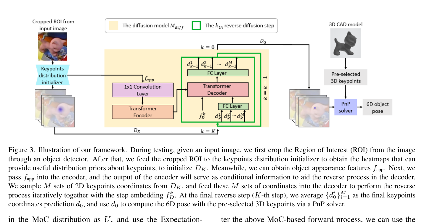
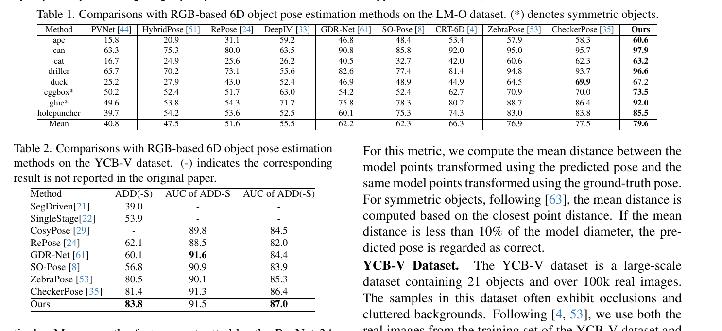
Original paper, Figure 3: The ROI first produces keypoint heatmaps and appearance features. A Mixture-of-Cauchy distribution initializes diffusion; a Transformer decoder iteratively recovers 2D keypoints, and the resulting 2D–3D correspondences enter PnP. Source: Official CVPR 2024 paper. Image copyright belongs to the authors and IEEE/CVF; shown here solely for paper analysis.Original paper, Tables 1–2: Mean ADD(-S) on LM-O is 79.6. YCB-V ADD(-S), ADD-S AUC, and ADD(-S) AUC are 83.8, 91.5, and 87.0, respectively. Source: Official CVPR 2024 paper. Table copyright belongs to the authors and IEEE/CVF; shown here solely for paper analysis.
4. Problem setting
Input: One RGB image, detected object ROI, known-instance CAD, and camera intrinsics.
Intermediate representation: 128 3D keypoints sampled from the CAD surface by FPS, with corresponding 2D heatmaps.
Output: Object-to-camera rotation and translation; scale is not predicted.
Protocol: Known-instance, model-based, RGB-only; requires an object detector and CAD.
Data: LM-O and YCB-Video; training mixes real images and publicly available PBR images.
5. Method overview
A ResNet-34 initializer predicts a heatmap for each keypoint from a 256×256 ROI and extracts appearance features.
Sample candidate coordinates from the heatmaps and fit the initial distribution DK with a mixture of 9 Cauchy kernels.
During training, progressively diffuse ground-truth 2D coordinates D0 toward the fitted heavy-tailed distribution to generate supervision at each step.
A three-layer Transformer encoder processes appearance; a three-layer decoder receives coordinates and diffusion-step embeddings to learn progressive reverse denoising.
At test time, sample 5 keypoint sets, use DDIM to reduce 100 training steps to 10 reverse steps, and average the final coordinates.
Pass 128 2D–3D correspondences to Progressive-X PnP to recover 6D pose.
6. Experiments at a glance
Mean LM-O ADD(-S): 79.6, versus 77.5 for CheckerPose and 76.9 for ZebraPose.
LM-O per object: ape 60.6, can 97.9, cat 63.2, driller 96.6, duck 67.2, eggbox 73.5, glue 92.0, holepuncher 85.5.
Standard Gaussian diffusion: 73.1; using heatmaps only as conditioning: 76.2; full MoC: 79.6.
Three direct-regression variants without progressive denoising: 49.2 / 57.3 / 61.1, all far below 79.6.
7. Quick assessment
Strength: Diffusion operates in interpretable 2D keypoint space, retaining constraints from established geometric solvers.
Strongest evidence: MoC outperforms standard Gaussian diffusion by 6.5 points, suggesting that heatmap-derived heavy tails and multiple modes better suit pose correspondences than generation from white noise.
Common misreading: It does not directly generate a multimodal SE(3) distribution; the final 5 coordinate sets are averaged into one solution.
Limitations: Requires object-specific CAD, detection boxes, instance training, and PnP. Training with 100 diffusion steps and inference with 10 steps are also more complex than one-pass regression.
Audience: RGB-only instance pose, keypoints/PnP, diffusion models, and correspondence uncertainty under occlusion.
Available src/paper-notes/6d-diff-cvpr2024/deep.md
In-depth paper notes
Support reproduction, comparison, related-work writing, and identifying opportunities for further research.
Deep Reading Notes: 6D-Diff
1. Key assessment
6D-Diff’s key contribution is choosing what to diffuse. Directly diffusing rotation and translation raises issues with SO(3) geometry, mismatched scales, and symmetric multiple solutions. The paper instead models N×2 2D keypoint coordinates, extracting uncertainty from network heatmaps while leaving final pose recovery to PnP.
More importantly, the reverse process does not start from a standard Gaussian. Occlusion, background interference, and self-occlusion often produce multimodal heatmaps with outlier tails; a Mixture-of-Cauchy (MoC) better represents this distribution than a Gaussian. Standard diffusion scores 73.1, heatmap-as-condition 76.2, and full MoC 79.6. These results support the data-dependent heatmap distribution as the diffusion endpoint, beyond simply increasing network depth.
2. Task Boundaries and Data Flow
Given ROI image I, a CAD model, and camera intrinsics, first select N=128 3D keypoints from the CAD surface by farthest point sampling:
X={xi∈R3}i=1N.
The goal is to predict their 2D projections:
d0={ui∈R2}i=1N,
Then solve:
(R,t)=PnP(X,d0,Kcam).
The method therefore uses:
known CAD, known instance;
Absolute pose from a single RGB image;
Correspondence-based estimation rather than direct pose regression;
No solution for detection, category discovery, unknown-object generalization, or scale estimation.
3. Why a Mixture-of-Cauchy?
The initializer outputs heatmap Hi for each keypoint. After sampling V coordinate sets from these heatmaps, fit U=9 Cauchy kernels:
ηMoC⋆=EM(v=1∏Vu=1∑UπuCauchy(dKv∣μu,γu)).
Cauchy tails are heavier than Gaussian tails, allowing a few background peaks or incorrect high responses without increasing the entire distribution’s variance; the mixture also retains multiple local peaks. This directly reflects the task:
Visible keypoint: a concentrated heatmap with high weight on one kernel;
Occluded keypoint: several candidate peaks coexist;
Background interference: a few distant outliers occupy the heavy tails;
Symmetry or nearly repeated textures: multiple kernels represent local modes.
MoC does not explicitly label which peaks are symmetry-equivalent solutions. The appearance-conditioned decoder and training ground truth still steer the distribution toward one supervised solution.
4. Data-Dependent Forward Process
Ordinary DDPM makes dK approach N(0,I). 6D-Diff instead makes the endpoint approach the fitted MoC:
d^k=αˉkd0+(1−αˉk)μMoC+1−αˉkϵMoC.
As αˉK→0, d^K approaches the heatmap-derived MoC. The forward process generates stepwise supervision only during training. At test time, samples are drawn directly from the initializer’s DK and processed in reverse, avoiding a mismatch between white-noise training starts and network-heatmap test starts.
5. Network and Training
Original paper, Figure 3. Yellow denotes the diffusion model, and green arrows mark progressive reverse steps. The model corrects only 2D keypoints; Progressive-X PnP still performs final geometric recovery. Source: Official CVPR 2024 paper. Image copyright belongs to the authors and IEEE/CVF; shown here solely for paper analysis.
Training has two stages:
Initializer: ResNet-34 followed by two deconvolution layers and a 1×1 convolution learns 128 heatmaps with L2 heatmap loss;
Diffusion model: A three-layer Transformer encoder processes appearance features. At each step, coordinate embeddings and sinusoidal step embeddings enter a three-layer decoder, whose cross-attention reads image context to regress the preceding coordinates.
The reverse loss supervises all 5 sample sets across 100 steps:
The implementation uses a V100, M=5, K=100, and 9 Cauchy kernels. The diffusion model trains for 1,500 epochs with Adam and an initial learning rate of 4×10⁻⁵. DDIM reduces test inference to 10 steps.
6. Does Progressive Denoising Actually Occur?
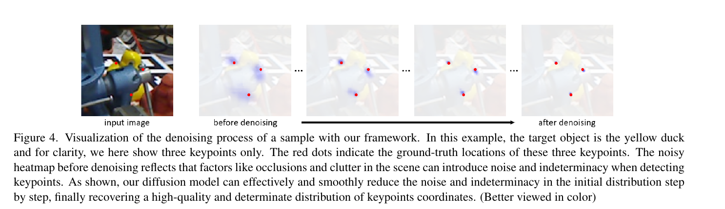
Original paper, Figure 4: Three keypoints are shown on the yellow-duck example. Initial heatmaps are diffuse with incorrect peaks; reverse steps progressively concentrate probability mass near the red ground-truth points. Source: Official CVPR 2024 paper. Image copyright belongs to the authors and IEEE/CVF; shown here solely for paper analysis.
The direct-regression comparison is essential:
Configuration
LM-O ADD(-S)
Variant A: coordinates directly from heatmaps
49.2
Variant B: same architecture with direct coordinate regression
57.3
Variant C: stacked to roughly match computation
61.1
Full progressive diffusion
79.6
Variant C controls for network depth and computation but still trails by 18.5 points, supporting the authors’ interpretation that progressive distribution transformation itself is useful. However, the paper provides neither per-reverse-step error curves nor the speed–accuracy trade-off across 1/5/10 steps.
7. Main results
Original paper, Tables 1–2. LM-O uses ADD(-S); YCB-V reports both threshold accuracy and AUC truncated at 10 cm. The three columns are not interchangeable. Source: Official CVPR 2024 paper. Table copyright belongs to the authors and IEEE/CVF; shown here solely for paper analysis.
LM-O
Method
Mean ADD(-S)
CRT-6D
66.3
ZebraPose
76.9
CheckerPose
77.5
6D-Diff
79.6
6D-Diff leads or shows clear advantages on can, cat, driller, eggbox, glue, and holepuncher. Its duck score is 67.2, below CheckerPose’s 69.9, so diffusion does not improve every object. The mean gain over CheckerPose is 2.1 points, a consistent improvement rather than an order-of-magnitude change.
YCB-Video
Method
ADD(-S)
ADD-S AUC
ADD(-S) AUC
ZebraPose
80.5
90.1
85.3
CheckerPose
81.4
91.3
86.4
6D-Diff
83.8
91.5
87.0
ADD-S AUC exceeds CheckerPose by only 0.2; clearer gains appear in ADD(-S) threshold accuracy (+2.4) and ADD(-S) AUC (+0.6).
8. Appearance and MoC Ablations
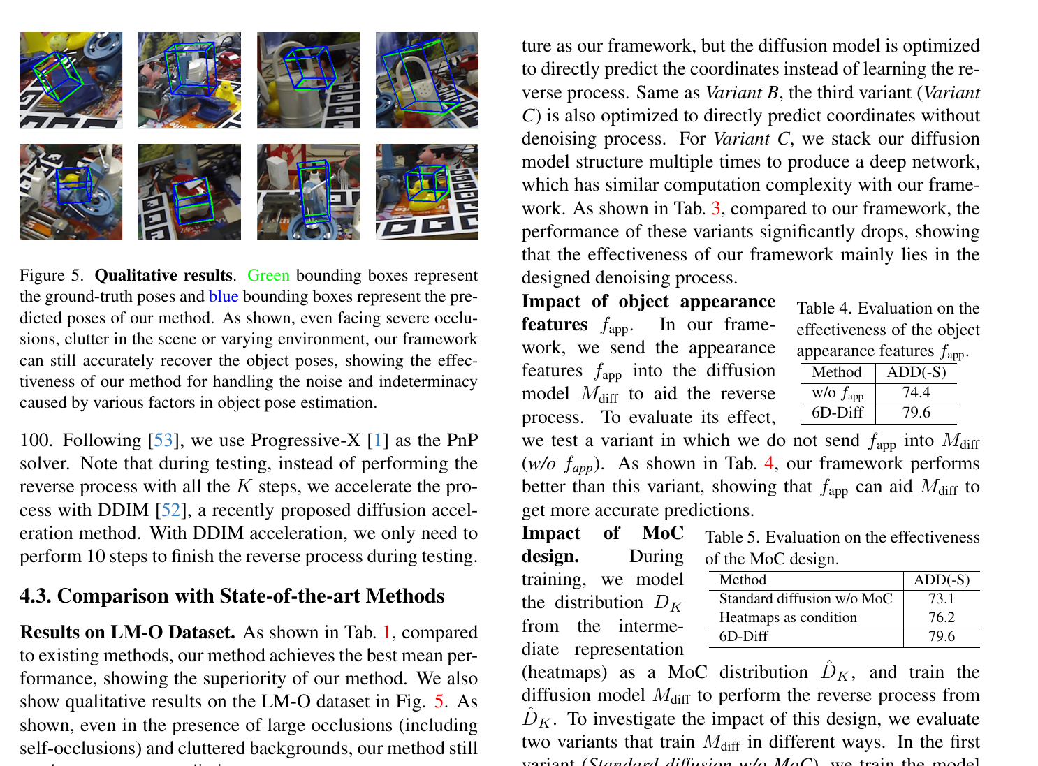
Original paper, Figure 5 and Tables 3–5: The left shows occluded LM-O scenes; the right separates the contributions of progressive denoising, appearance conditioning, and MoC initialization. Source: Official CVPR 2024 paper. Image and table copyright belongs to the authors and IEEE/CVF; shown here solely for paper analysis.
Design
LM-O ADD(-S)
Difference from full model
No appearance features
74.4
-5.2
Standard Gaussian diffusion, no MoC
73.1
-6.5
Gaussian initialization + heatmap conditioning
76.2
-3.4
MoC initialization + appearance conditioning
79.6
—
MoC contributes more than appearance conditioning, but they are complementary: MoC defines the initial coordinate distribution, while appearance guides each step. Conditioning on a heatmap differs from using it as the starting distribution.
9. Limits of the Uncertainty Interpretation
The paper repeatedly discusses noise and indeterminacy, but the output is collapsed to one solution three times:
The 5 reverse sample sets are averaged in coordinate space;
These per-keypoint means form one deterministic correspondence set;
PnP outputs one pose.
6D-Diff therefore uses distributions for robust point estimation rather than producing a calibrated pose posterior. For strongly symmetric objects, coordinate means may even lie between valid modes. The paper evaluates with ADD-S but shows neither multimodal pose samples nor confidence calibration.
10. Reproduction and Limitations
Faster R-CNN / FCOS boxes come from CDPNv2; detection errors are not reported separately from keypoint diffusion.
LM-O uses LM real + PBR, and YCB-V uses real + PBR; training is not real-only.
Each instance needs CAD, 3D keypoints, and object-specific training; novel objects are unsupported.
Progressive-X is more robust than ordinary PnP; final scores include the robust solver’s contribution.
The paper reports no end-to-end FPS, parameter count, or memory usage; the deployment cost of 10 decoder passes requires measurement.
MoC fitting uses EM, making training more complex than standard heatmap regression.
The paper does not compare Laplace, Student-t, Gaussian mixtures, or other heavy-tailed alternatives, so Cauchy cannot be declared uniquely optimal.
11. Overall assessment
6D-Diff offers clear problem modeling for diffusion-based pose estimation. It retains the geometric interpretability of correspondence + PnP and uses diffusion for the unstable 2D keypoint-localization stage. MoC and direct-regression ablations support the central design, with consistent gains on LM-O / YCB-V.
Its boundaries are equally clear: known CAD, a single solution, no speed report, and no explicit modeling of symmetric multimodal distributions on SE(3). A valuable extension would retain multiple keypoint samples through pose-hypothesis generation and jointly evaluate symmetry-aware likelihoods, PnP uncertainty, and few-step sampling.