Differentiable Rendering-based Pose Estimation for Surgical Robotic Instruments
From a single endoscopic RGB image, SAM2 mask, dVRK CAD / kinematics, and inaccurate joint angles, the method batch-optimizes 500 initializations in a four-dimensional LookAt space, then jointly refines camera-to-robot extrinsics and three distal joints. Results on 30 real frames improve RCM geometric consistency, without absolute extrinsic ground truth or runtime results. It initializes a markerless tracker rather than providing real-time tracking.
One 640×480 monocular endoscopic image, SAM2 mask, dVRK CAD / kinematics, and inaccurate encoder joints initialize 500 candidates in a four-dimensional RCM-constrained space. Differentiable refinement jointly estimates camera–robot extrinsics and three visible joints. This initializes markerless tracking, with no real-time claim or absolute extrinsic GT.
3. Guide to figures and tables
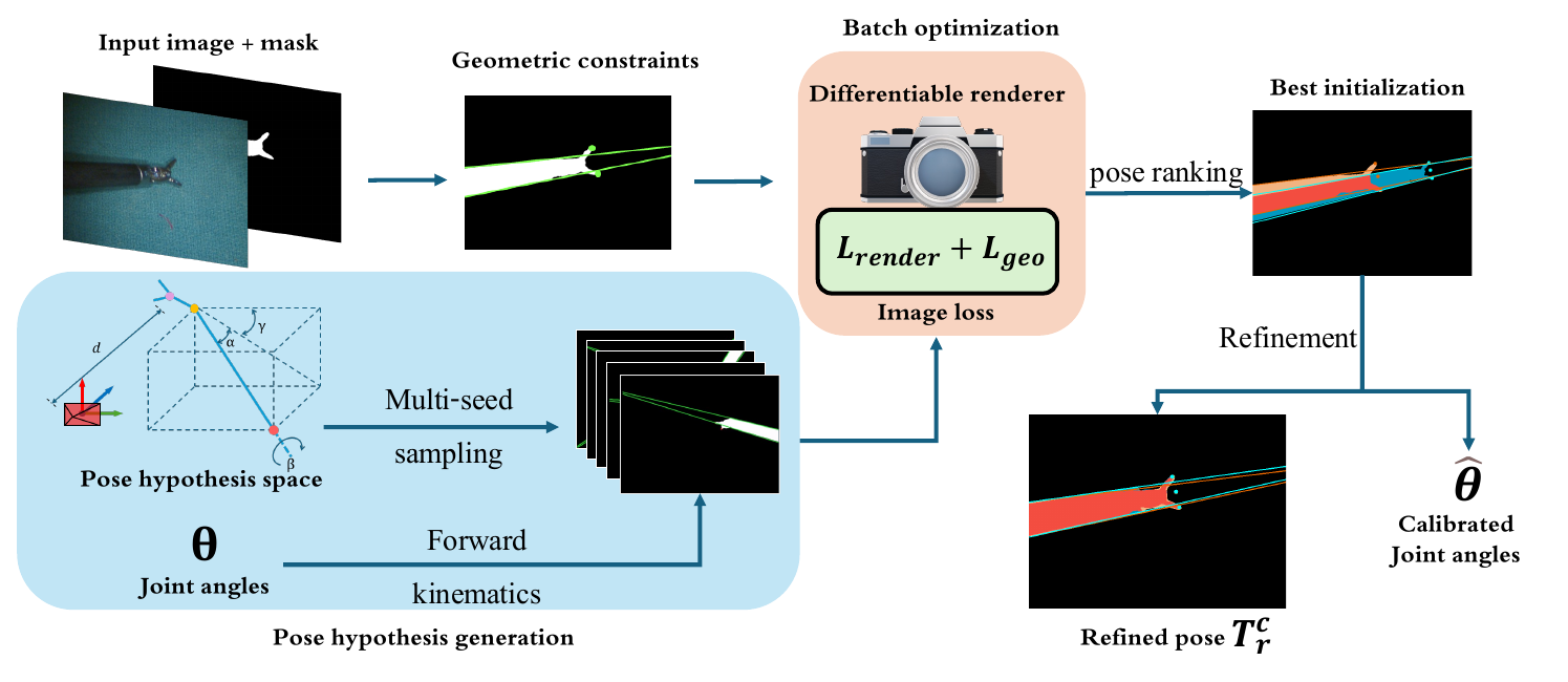
Original Figure 2: low-resolution images, masks, and inaccurate joints generate specialized hypotheses; rendering / geometry losses rank them before joint extrinsic / distal-angle refinement. Source: authors' public manuscript. Image copyright belongs to the authors and IEEE; reproduced here for paper analysis.Original Figures 6–7 and Tables I–II: 30 real frames grouped by difficulty show lower RCM-convergence distance standard deviations than PnP. Gauze grasps remain stable while needle success declines with distance. This measures cross-frame consistency, without GT extrinsic rotation / translation errors. Source: authors' public manuscript. Image / table copyright belongs to the authors and IEEE; reproduced here for paper analysis.
4. Problem setting
Platform: dVRK Patient Side Manipulator (PSM), large needle driver.
Inputs: monocular RGB, SAM2 binary tool mask, intrinsics, link meshes / CAD, and encoder joint estimates.
Outputs: transform Trc mapping robot base to camera in the rendering equation, termed camera-to-robot by the paper, plus calibrated Wrist Pitch, Wrist Yaw, and Jaw Angle.
Prior: Remote Center of Motion constrains the insertion axis; images typically show a long shaft and tiny gripper.
Single-shot means one image. Each frame still optimizes 500 candidates for 100 coarse steps, then the best for 1000 refinement steps. Unreported runtime prevents one-pass / real-time interpretations.
5. Method overview
Obtain SAM2 reference silhouettes.
Parameterize poses as [α,β,γ,d]: two camera-relative angles, shaft roll, and camera–origin distance.
Render dVRK kinematics / meshes through PyTorch3D silhouettes.
Compare mask MSE, distance fields, and mask-area scale.
Add projected shaft-edge line losses and gripper-tip keypoints for narrow structures.
After 100 batch steps, refine the best for 1000 steps with Gaussian perturbations / coordinate descent, jointly calibrating three distal joints.
6. Why silhouette MSE alone is insufficient
Disjoint masks provide little directional gradient under ordinary MSE.
Reference-mask distance fields extend gradients across the image.
Area differences constrain coarse depth / scale.
Narrow shaft orientation barely changes total mask area; Canny / Hough edges supply explicit line constraints.
Two tip keypoints constrain gripper opening / orientation.
Silhouettes constrain visible regions while analytical geometry addresses poorly conditioned directions, rather than directly regressing RGB poses.
7. Experiments at a glance
Calibration consistency
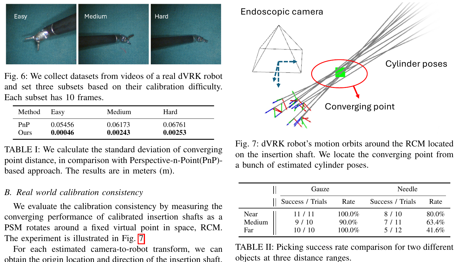
Easy / medium / hard videos each supply 10 frames. Estimated shaft axes define distances to a common RCM; compare distance standard deviations:
Method
Easy ↓
Medium ↓
Hard ↓
PnP
0.05456 m
0.06173 m
0.06761 m
Ours
0.00046 m
0.00243 m
0.00253 m
These support fixed-RCM consistency, without external mocap / fiducial GT for absolute extrinsic errors. Shared systematic bias can preserve good convergence.
Open-loop grasping
Distance
Gauze
Needle
Near, about 1 cm
11 / 11, 100%
8 / 10, 80%
Medium, about 3–4 cm
9 / 10, 90%
7 / 11, printed as 63.4%
Far, about 7 cm
10 / 10, 100%
5 / 12, 41.6%
7/11 is about 63.6%, inconsistent with printed 63.4%. Gauze targets use ArUco / PnP, and needle targets an existing tracker. Success mixes target pose, open-loop control, encoder errors, and grasp geometry rather than isolating calibration.
8. Quick assessment
Highlight: shaft / gripper / RCM structure shapes sampling and losses, reducing arbitrary-SE(3) local minima.
Practical advantage over PnP: no tool paint / markers or sole reliance on low-resolution keypoint matches.
In original Eq. (4), Trc maps robot-base coordinates to camera coordinates, despite the paper’s camera-to-robot name. Forward kinematics Tmr(θ) maps meshes to robot base; M are known link meshes, R the silhouette renderer, and Mref the endoscopic tool mask.
Cable stretch / hysteresis corrupt joints; only a small shaft / gripper segment is visible; arbitrary-SE(3) silhouette fitting has local minima. The contribution combines specialized search, rendering, and analytical geometry for single-frame initialization.
2. Inputs, outputs, and boundaries
Original Figure 2: 500 starts undergo batch ranking; the best receives longer refinement. Outputs include extrinsics, Wrist Pitch, Wrist Yaw, and Jaw Angle. Source: authors' public manuscript. Image copyright belongs to the authors and IEEE; reproduced here for paper analysis.
Required inputs
One 640×480 monocular endoscopic RGB image;
Reference mask from Segment Anything 2;
camera intrinsics;
Metric dVRK link meshes / CAD;
dVRK forward-kinematics model;
Approximate encoder joints;
Hypothesis ranges suited to real dVRK scenes.
Outputs
Robot-base-to-camera transform Trc;
Calibrated Wrist Pitch, Wrist Yaw, and Jaw Angle.
Outside scope
Unknown-tool / unknown-CAD category transfer;
General 6D pose without robot kinematics;
Temporal filtering / online drift correction;
Gauze / needle target pose estimation;
Absolute calibration GT.
Markerless refers to the tool. Gauze experiments still use target ArUco markers, so the full manipulation system is not marker-free.
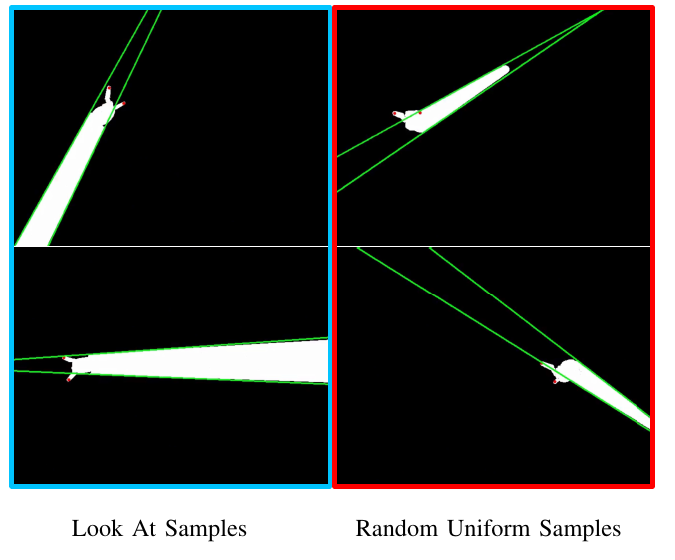
Original Figure 4: LookAt focuses starts on feasible front-facing instruments, while uniform 6D samples waste candidates. This qualitative comparison lacks hypothesis recall or count–accuracy curves. Source: authors' public manuscript. Image copyright belongs to the authors and IEEE; reproduced here for paper analysis.
Instead of sampling unbounded SE(3), the authors use:
The insertion shaft should face the workspace, excluding camera-back / intersecting configurations. This lets 500 candidates cover useful regions under dVRK / RCM geometry, without constituting a general articulated-object parameterization.
The mechanism plausibly helps speed / accuracy, but tables cannot isolate its quantitative contribution.
4. Kinematics and differentiable silhouettes
Transform mesh vertices into camera coordinates through kinematics and candidate extrinsics:
vc=TLookAtTmr(q)vm.
PyTorch3D renders visible links into binary mask S. This:
Differentiates extrinsics and visible joints jointly;
Avoids texture / material / lighting matches between simulation and reality.
Quality is limited by masks, CAD, and kinematics. Missing gripper pixels, highlights, or included background bias the objective. Qualitative mask examples lack perturbation curves or GT-mask comparisons.
5. Three rendering losses
5.1 Silhouette MSE
LMSE=i,j∑(S(i,j)−Mref(i,j))2.
Mask MSE supports overlapping fine alignment but gives poor directional gradients at large separations.
5.2 Distance-field loss
Reference distance field Dref extends background values with distance to the foreground:
Ldist=i,j∑S(i,j)Dref(i,j).
Even disjoint rendered foreground moves toward the reference, enlarging convergence basins.
5.3 Scale loss
Lscale=i,j∑S(i,j)−i,j∑Mref(i,j).
Area depends on depth d, supplying coarse camera-distance constraints. Different depths, shaft angles, and joints can still share an area.
Combined rendering loss:
Lrender=λ1LMSE+λ2Ldist+λ3Lscale.
Complete λi weights, field decay, and scale sensitivity are undisclosed, leaving reproduction gaps.
6. Why analytical geometry matters
Long, narrow shafts dominate visible area. Small orientation errors matter for control while changing few mask pixels.
6.1 Cylinder edge loss
Known-radius cylinders define two projected edges. Canny / Hough recover the longest reference lines, represented in polar coordinates (ρ,θ):
d(ℓ1,ℓ2)=min(∣θ1−θ2∣,π−∣θ1−θ2∣)+γ∣ρ1−ρ2∣.
Loss evaluates both edge assignments and their mean differences:
Automatic reference-tip extraction is unclear. SAM2 directly supplies masks, leaving this a reproduction question.
Final objective:
L=Lrender+Lgeo,Lgeo=λ4Lcylinder+λ5Lkpt.
7. Two-stage optimization beyond a forward pass
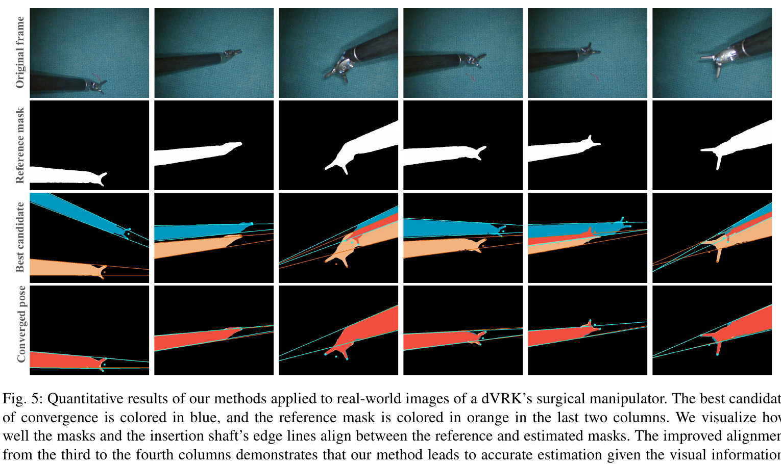
Original Figure 5: each column contains an image, reference mask, ranked candidate, and converged result; blue is the estimated projection and orange the reference. Despite the original caption's quantitative label, this visualizes alignment without numerical errors. Source: authors' public manuscript. Image copyright belongs to the authors and IEEE; reproduced here for paper analysis.
On RTX 3090:
Input: 640×480;
500 candidates per frame;
Coarse: 100 Adam iterations each, learning rate 0.003;
Gaussian perturbations and coordinate descent during refinement;
Joint Wrist Pitch, Wrist Yaw, and Jaw Angle optimization.
About 50,000 candidate-iterations plus 1000 refinement steps lack wall-clock, memory, batch-size, success-rate, or stopping reports. Thus:
Single-shot / one-shot means one image;
It does not mean one pass;
It does not establish real-time operation;
Few coarse iterations do not determine engineering latency.
Active tracking and real-time joint-error correction remain future work.
8. Calibration consistency is not absolute error
Original Figures 6–7 and Tables I–II. Left: real data / RCM consistency with 10 frames per level. Right: convergence geometry and open-loop grasping. Source: authors' public manuscript. Image / table copyright belongs to the authors and IEEE; reproduced here for paper analysis.
PSM motions orbit a fixed RCM. For estimated shaft i with origin pi and direction di, find the point minimizing total distance to the axes:
x∗=argxmini∑(x−pi)−(di⊤(x−pi))di2.
Then measure distance standard deviation σ:
Method
Easy ↓
Medium ↓
Hard ↓
PnP
0.05456 m
0.06173 m
0.06761 m
Ours
0.00046 m
0.00243 m
0.00253 m
Relative to PnP, standard deviations fall about 96%–99% across levels, showing axes close to a shared RCM. This is strong geometry evidence for RCM-constrained dVRK.
It does not measure:
camera-to-robot translation error;
rotation error;
ADD / ADD-S;
Error against external mocap / fiducial calibration GT.
Shared systematic extrinsic bias can still yield consistent convergence. Only 3×10=30 frames are tested, without video / camera-placement counts, sampling details, or operational difficulty definitions. Evidence supports better RCM consistency, without proving absolute 0.46 mm calibration.
9. Interpreting open-loop manipulation
Using one initial calibration, random PSM / target starts execute:
Move above target → approach and pick → place → reset.
Distance groups: about 1 cm, 3–4 cm, and 7 cm:
Distance
Gauze success
Needle success
Near
11 / 11 = 100%
8 / 10 = 80%
Medium
9 / 10 = 90%
7 / 11; printed 63.4%
Far
10 / 10 = 100%
5 / 12 = 41.6%
Four boundaries matter:
7/11=63.636…% normally rounds to 63.6%; printed 63.4% appears inconsistent.
Gauze targets use attached ArUco / OpenCV PnP; markerless tool calibration does not make target localization markerless.
An existing real-time needle tracker supplies needle poses.
Gauze is large / tolerant, with near-100% performance across distances; needles are less tolerant, and accumulated errors reduce 80% to 41.6%. One calibration cannot replace online feedback, motivating active tracking.
10. Relationship to PnP initialization
Earlier dVRK trackers use painted or detected 2D features and robot-model points for PnP. Challenges include:
Low endoscopic resolution, lighting, and reflections;
Tiny gripper features;
Pixel-sensitive 2D–3D associations;
Extra physical markers in some systems;
Too few points under image cropping.
This method combines:
Global silhouettes;
Long-range distance-field gradients;
shaft cylinder edges;
gripper tips;
dVRK kinematics;
RCM-compatible candidate space.
Tip keypoints remain in geometry loss alongside cylinder edges / silhouettes. The change is joint evidence beyond sparse keypoint-only PnP, rather than eliminating keypoints.
As of 2026-07-31, no public author code / evaluation data was found. Algorithmic reconstruction remains possible, with insufficient detail for unambiguous numerical reproduction.
12. Limitations
Strong dVRK CAD, kinematics, RCM, and visible-geometry priors;
One PSM / large needle driver, without cross-tool tests;
SAM2 dependence without quantified mask robustness;
500×100 + 1000 optimization steps without runtime;
Unspecified sampling ranges, coverage, and quantitative ablations;
Missing loss weights / thresholds;
Consistency rather than absolute calibration GT;
Only 30 real frames;
Mainly keypoint-PnP comparison, without marker GT or alternative render-and-compare baselines;
Target / control errors mixed into grasp success;
Target ArUco in gauze experiments;
Far-needle success only 41.6%;
Inconsistent printed percentage for 7/11;
Single-frame initialization without online correction;
Unreleased code / evaluation data.
13. Overall assessment
The modeling closely fits surgical mechanics: partial end-effector visibility, cylindrical shafts, RCM motion, and inaccurate encoders structure global candidate ranking plus local joint refinement.
The strongest evidence is more consistent RCM geometry than PnP on 30 real frames, with one initialization supporting some open-loop grasps. Submillimeter absolute calibration, real-time operation, and entirely marker-free manipulation remain unproven. Absolute GT, runtime, ablations, and online tracking would strengthen this surgical-robot vision-calibration approach.