Category-Level Object Shape and Pose Estimation in Less Than a Millisecond
The paper formulates category-level shape–pose MAP conditions as a nonlinear eigenproblem over unit quaternions. SCF iterations require only a minimum eigenvector of a 4×4 matrix per step for local solutions, and Lagrangian duality checks global optimality. A synthetic solve takes around 0.12 ms and the REAL275 solver around 1.26 ms, excluding roughly 50 ms of frontend keypoint detection.
category-specific semantic keypoint detectordepth for lifting keypoints to 3Dlinear active shape modelcorrect keypoint correspondences or a robust wrapper
Full paper metadataAuthors, affiliations, research area, datasets, metrics, method tags, and reading statusExpandCollapse
Authors
Lorenzo Shaikewitz, Tim Nguyen, Luca Carlone
Affiliations
MIT Laboratory for Information and Decision Systems / Boston University / MIT SPARK Lab
category-specific semantic keypoint detectordepth for lifting keypoints to 3Dlinear active shape modelcorrect keypoint correspondences or a robust wrapper
Reading Notes
Overview / Deep Dive
Available src/paper-notes/category-shape-pose-millisecond-icra2026/coarse.md
Paper overview notes
Quickly assess the paper's scope, problem setting, core method, experimental findings, and whether to read it in depth.
Paper Overview: Category-Level Object Shape and Pose Estimation in Less Than a Millisecond
Authors / affiliations: Lorenzo Shaikewitz, Tim Nguyen, Luca Carlone; MIT LIDS / SPARK, Boston University.
Task: Jointly estimate shape coefficients, rotation, and translation from a known category shape library and semantic 3D keypoints detected by an RGB-D frontend.
2. Positioning in one sentence
The paper reduces category-level shape–pose MAP estimation to a self-consistent eigenproblem over unit quaternions. Each SCF update constructs a 4×4 matrix and selects its smallest eigenvector, followed by an inexpensive dual check that can certify global optimality.
3. Method overview
A linear active shape model represents each semantic keypoint as a combination of corresponding training-shape points, with priors on the coefficients. After eliminating translation and shape variables, the rotation quaternion q satisfies an eigen-equation that depends on q itself. Self-consistent field (SCF) iteration proceeds as follows:
Use the current qt to construct a symmetric 4×4 matrix.
Use the unit eigenvector associated with its smallest eigenvalue as qt+1.
After convergence, back-substitute shape and translation.
Solve a linear system for Lagrange multipliers and check that the dual matrix is positive semidefinite. Passing yields an a posteriori global-optimality certificate.
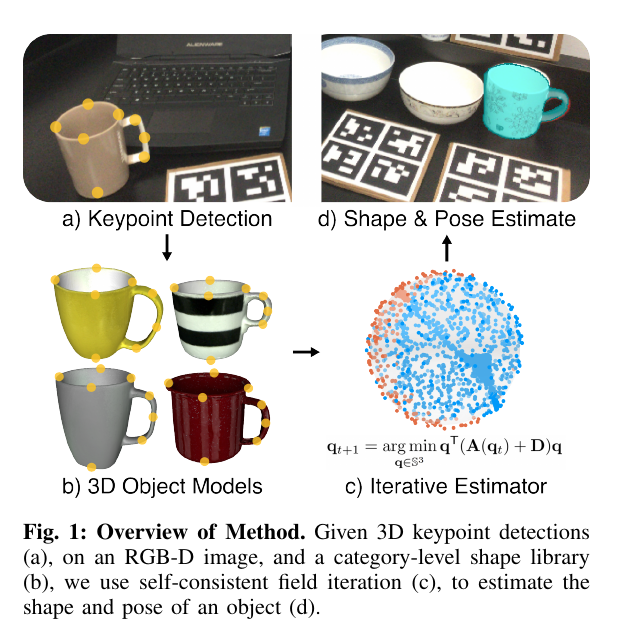
Original paper, Figure 1: An RGB-D frontend supplies semantic 3D keypoints, a linear category shape library supplies priors, and the SCF backend jointly recovers shape and pose. Source: original paper. Copyright belongs to the paper's authors; reproduced here solely for academic discussion.
4. Experiments at a glance
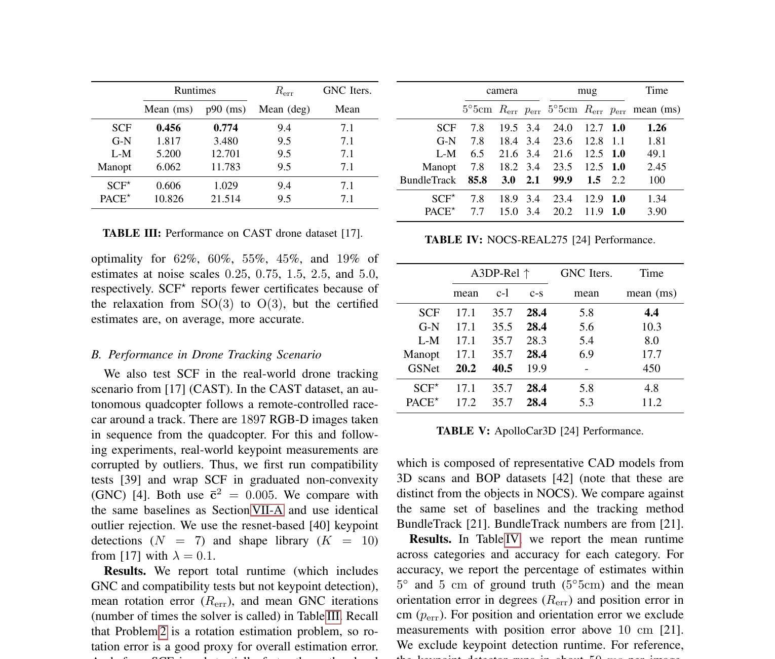
Synthetic problems: SCF takes approximately 0.104–0.108 ms, certified SCF* 0.120–0.126 ms, GN / LM 0.2–0.3 ms, and PACE* 1.66 ms.
CAST: SCF averages 0.456 ms with 9.4° rotation error; GN takes 1.817 ms and PACE* 10.826 ms.
NOCS REAL275 camera / mug experiments: SCF averages approximately 1.26 ms, but the keypoint detector takes approximately 50 ms, as the paper explicitly states.
ApolloCar3D: SCF takes approximately 4.4 ms, with A3DP mean / c-l / c-s of 17.1 / 35.7 / 28.4. Slower GSNet is more accurate, and hardware and detector inclusion differ across comparisons.
Original paper, Tables III–V: Real-data results require distinguishing backend-solver time from frontend-detector time. Baselines may also differ in hardware and end-to-end timing scope. Source: original paper. Copyright belongs to the paper's authors; reproduced here solely for academic discussion.
5. Quick assessment
Highlight: Combines speed and verifiability, suiting repeated hypotheses within RANSAC / GNC.
Essential timing scope: Less than a millisecond refers to typical core-solver problem sizes, not the complete RGB-D-to-pose system.
Limitations: Requires the correct category, semantic keypoint correspondences, depth, and a linear shape library. Certificate failure means global optimality is unproven; it does not automatically repair incorrect observations.
Available src/paper-notes/category-shape-pose-millisecond-icra2026/deep.md
In-depth paper notes
Support reproduction, comparison, related-work writing, and identifying opportunities for further research.
Deep Reading Notes: Category-Level Object Shape and Pose Estimation in Less Than a Millisecond
Key problem: Joint category-level shape–pose estimation is nonconvex and must handle outliers. Certifiable SDP methods are expensive, while local Gauss–Newton offers no optimality guarantee. Can a fast solver with a posteriori certification bridge this gap?
Main answer: First-order unit-quaternion optimality conditions yield a self-consistent field eigenproblem. Each step computes the smallest eigenvector of a 4×4 matrix; dual KKT conditions check global optimality after convergence.
My assessment: This is a geometric-solver paper rather than an end-to-end vision system. Its most useful measure is cost per hypothesis / backend solve, making it suitable for GNC, compatibility tests, and sampling-based robust estimation. A single 0.1 ms solve should not be compared directly with full-network FPS.
2. Positioning in one sentence
Fast-ShapeAndPose turns nonconvex category-level shape–pose optimization into a sequence of 4×4 eigensolves through SCF, replacing an expensive SDP global-optimality check with a linear system and a positive-semidefiniteness test.
2.1 Guide to figures and tables
Figure / table
What to look for
Figure 1
Inputs are already semantic 3D keypoints; the visual frontend is outside the submillisecond solver.
Algorithm 1
SCF updates are short; the difficulty lies in deriving A(qq⊤)+D and understanding fixed-point properties.
Tables I–II
Solver-only latency and solution quality of local / certifiable versions under synthetic conditions.
Tables III–V
CAST, REAL275, and ApolloCar3D use different system scopes; read accuracy, frontend, and hardware notes together.
Original paper, Figure 1: Yellow points are semantic 3D keypoints detected by the visual frontend and lifted through depth. SCF only recovers instance shape and pose from these points and the shape library. Source: original paper. Copyright belongs to the paper's authors; reproduced here solely for academic discussion.
3. Mathematical problem
Suppose a category has K training shapes, each defining N semantically corresponding keypoints. Model point i of an unknown instance uses a linear active shape model:
si(c)=k=1∑Kckbk,i,
Here c contains shape coefficients, typically with ∑kck=1 or Gaussian / quadratic regularization. The RGB-D frontend supplies camera-frame 3D observations yi. The objective minimizes:
i∑wi∥yi−Rsi(c)−t∥2+λ∥c∥2,
Jointly solve for R∈SO(3), t, and c.
There are three difficulties:
Orthogonality of R makes the problem nonconvex.
Multiplication of R and c couples shape and pose.
Real keypoint detectors miss or mismatch points, requiring a robust outer loop.
PACE* uses semidefinite relaxation for certifiable solutions, but solving an SDP per RANSAC / GNC hypothesis is costly. GN / LM are fast but converge to initialization-dependent local solutions.
4. Elimination and quaternion formulation
Translation t can be eliminated in closed form by centering observations and model points. With rotation fixed, shape coefficients c solve linear least squares with quadratic regularization and can be expressed as a function of rotation. Only rotation remains in the objective.
The authors represent rotation with a unit quaternion q∈S3 for R. Rotated quadratic terms become quartic polynomials in q; first-order stationarity ultimately gives:
(A(qq⊤)+D)q=λq.
This resembles an eigenproblem, but the matrix depends on unknown q, so one eigendecomposition is insufficient. SCF freezes the matrix using current qt, then selects a new smallest eigenvector.
5. Local SCF solver
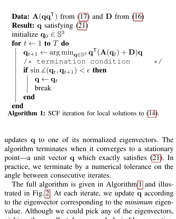
Original paper, Algorithm 1 and following explanation: Construct a matrix from the current quaternion and update with its smallest eigenvector until angular distance between successive quaternions falls below a threshold. Source: original paper. Copyright belongs to the paper's authors; reproduced here solely for academic discussion.
The algorithm is:
Start with a unit quaternion q0.
Compute Mt=A(qtqt⊤)+D.
Select the unit eigenvector of Mt associated with its smallest eigenvalue as qt+1.
Stop based on quaternion angular distance rather than ordinary Euclidean difference.
Back-substitute to obtain c,t.
Why the smallest eigenvector? At a stationary point, the objective can be written as the corresponding Rayleigh quotient, and local minima are typically governed by the smallest eigenpair. The matrix is only 4×4, so updates are inexpensive. Usually fewer than 5 iterations are observed; with 10 keypoints, a single-threaded C++ update can take less than 10 μs.
SCF remains local. Different initializations may reach different stationary points, and eigenvectors can flip sign. Since q and −q represent the same rotation, stopping criteria must handle the double cover.
6. Fast global-optimality certification
Instead of solving an SDP first, the authors certify a candidate returned by SCF a posteriori. The original problem is a QCQP, with a Shor-relaxation dual constructed from Lagrange multipliers. Given a candidate quaternion:
Solve a small linear system from KKT stationarity for the multipliers.
Construct the dual matrix.
Check positive semidefiniteness and agreement of primal / dual objectives.
Passing means the candidate attains the relaxation’s lower bound and is globally optimal for the original problem. Failure means only that optimality was not certified, not that the solution is necessarily wrong. A certificate is a reliability signal, not an automatic error corrector.
The certified version is SCF*. Its small additional cost allows certification after every local solve. On failure, a system can change initialization, remove suspicious correspondences, or acquire new observations.
7. Synthetic experiments: Solver-only performance
The paper compares SCF, Gauss–Newton, Levenberg–Marquardt, and PACE*. Typical results:
SCF: Approximately 0.104–0.108 ms.
SCF*: Approximately 0.120–0.126 ms.
GN / LM: Approximately 0.2–0.3 ms.
PACE*: Approximately 1.66 ms.
SCF achieves less than a millisecond at these controlled sizes, remaining well below 1 ms with certification. Timing starts from an already constructed problem and ends with shape / pose, excluding RGB-D networks, keypoint detection, image loading, and data transfer.
Synthetic ablations show that SCF usually reaches the same objective as certifiable global methods, but not every result is certified. Noise, shape-model mismatch, and initialization affect certification rates. Deployments should report accuracy, runtime, and certification rate together.
8. Real-data experiments
Original paper, Tables III–V: Three real-data settings test general shape–pose estimation, robust NOCS estimation, and vehicle pose. Hardware and timing scopes differ, preventing ranking solely by the smallest millisecond value. Source: original paper. Copyright belongs to the paper's authors; reproduced here solely for academic discussion.
8.1 CAST
On CAST, SCF averages approximately 0.456 ms with approximately 9.4° rotation error; GN takes 1.817 ms and PACE* 10.826 ms. Similar accuracy at much lower latency suggests little loss of solution quality from SCF’s numerical approximation for the given keypoints.
8.2 NOCS REAL275
The authors combine SCF with camera / mug keypoint frontends and a compatibility test. The solver averages approximately 1.26 ms, but the keypoint detector explicitly takes approximately 50 ms, so the complete system does not run at 1 kHz. Robust outer loops call the solver repeatedly; SCF keeps multiple-hypothesis / compatibility checks affordable.
Accuracy is similar to other local solvers rather than uniformly exceeding strong learned / tracking systems; BundleTrack, for example, has better relevant pose accuracy. The focus is backend speed and certification, not leadership on every end-to-end benchmark.
8.3 ApolloCar3D
SCF takes approximately 4.4 ms with A3DP mean / c-l / c-s of 17.1 / 35.7 / 28.4. GSNet reports approximately 450 ms and 20.2 / 40.5 / 19.9. SCF is faster and competitive on some metrics, but hardware, frontends, and timing scopes differ; this is not a controlled 102× speedup. Apollo also uses more keypoints / larger hypothesis workloads, exceeding 1 ms and confirming that the title describes typical solver sizes rather than an upper bound for every setting.
9. Authors’ claims and my assessment
Authors’ claims
My assessment
Shape–pose estimation below 1 ms
Holds for the main solver benchmarks; the REAL275 visual frontend takes approximately 50 ms and the Apollo setup approximately 4.4 ms.
Efficient global-optimality certification of local solutions
Mathematically supported with low overhead; only passing certificates carry the guarantee.
Suitable for fast outlier rejection
Persuasive because robust wrappers solve repeatedly; compatibility testing is demonstrated.
Competitive accuracy
Supported among solvers sharing keypoint inputs; frontend and shape priors primarily limit end-to-end accuracy.
10. Reproduction checklist
Validate the objective, quaternion signs, and shape-coefficient constraints on repository synthetic data before adding a visual frontend.
Compare SCF, GN, and LM from the same q0, recording objectives, pose errors, iteration counts, and certification rates.
Linear shape bases must share semantic-point topology. Missing keypoints require consistent weight / elimination-matrix changes.
Depth units, model scale, and regularization jointly affect translation / shape conditioning.
Use numerical tolerances for certificate PSD checks and report the minimum eigenvalue rather than only a Boolean.
Break end-to-end timing into detection, 3D lifting, robust-wrapper call count, SCF, and certification.
With GNC / RANSAC, report mean solver calls per frame; one 0.1 ms solve is not total robust-estimation time.
11. Limitations and implications
Category-keypoint dependence: Requires semantically consistent points across instances. Large topology changes or unstable part correspondences can invalidate the active shape model.
Linear shape space: A few linear bases may not capture strongly nonlinear deformation or multimodal category shapes.
Depth dependence: Inputs are 3D keypoints. The backend does not eliminate depth problems on transparent / reflective objects.
Certificate scope: Guarantees optimization globality for the given observations and model, not observation correctness, correct category, or coverage of the true instance by the shape library.
Frontend/backend coordination: Predict keypoint covariances, pass heteroscedastic weights into the solver, and let certification failures trigger new views or active perception.
The paper offers a practical reminder: End-to-end networks need not absorb every geometric computation. Given semantic 3D correspondences, a specialized small certifiable solver can be faster than general optimization and easier to diagnose than direct pose regression.