Physics-Based Rigid Body Object Tracking and Friction Filtering From RGB-D Videos
The method uses differentiable rigid-body simulation as the state transition of an Extended Kalman Filter, jointly tracking position, SO(3) rotation, velocity, and friction coefficients between RGB-D pose measurements.
RGB-D pose observationsknown object mass and meshcontact surface modeldifferentiable rigid-body simulator
Reading Notes
Overview / Deep Dive
Available src/paper-notes/physics-rigid-object-tracking-3dv2024/coarse.md
Paper overview notes
Quickly assess the paper's scope, problem setting, core method, experimental findings, and whether to read it in depth.
Physics-Based Rigid Object Tracking: Coarse Notes
One-sentence conclusion
A differentiable rigid simulator supplies the Extended Kalman Filter transition. An RGB-D pose detector supplies measurements; physics predicts through missed detections, collisions, and sliding while estimating velocity and friction from trajectories.
State and workflow
State comprises position, SO(3) rotation, linear / angular velocity, and friction. CIR measures RGB-D pose; a differentiable Newton–Euler / contact simulator predicts the next state and supplies EKF Jacobians through autodifferentiation. Missing detections trigger prediction alone, followed by correction when observations return.
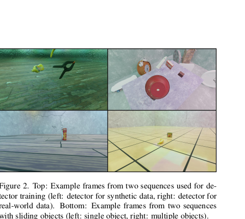
An RGB-D estimator for known meshes supplies observations; physics does not recognize objects directly. Source: original Figure 2. Copyright belongs to the authors and 3DV 2024 publisher; reproduced here for academic analysis.
Results
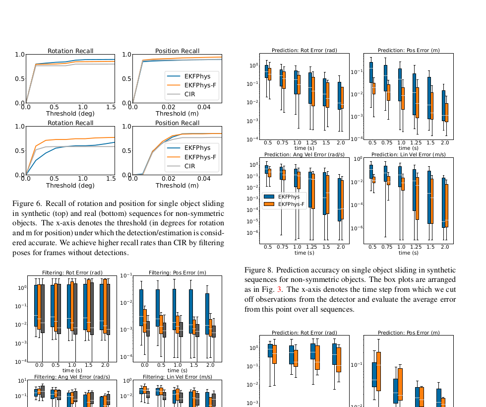
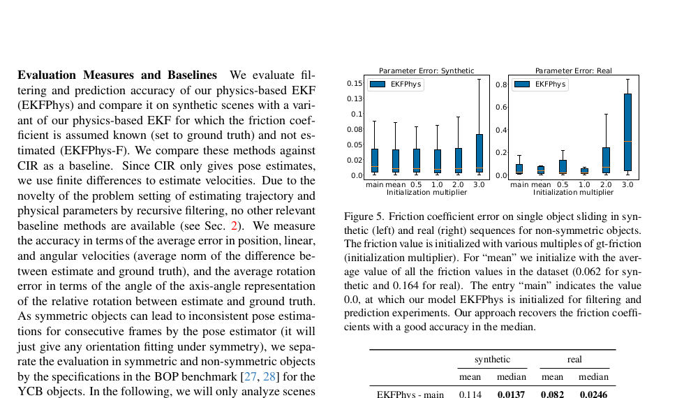
With friction initialized at zero, synthetic / real median absolute errors are 0.0137/0.0246, versus constant-zero baselines of 0.0192/0.03. Filtered rotation / position recall exceeds framewise CIR on missed detections; collision physics can propagate occluded objects.
Filtering is distinguished from prediction after observations stop. Velocity and friction need several observable-motion frames to converge. Source: original Figures 6–9. Copyright belongs to the authors and 3DV 2024 publisher; reproduced here for academic analysis.
Boundaries
Known meshes, masses, tabletop / contact models, and RGB-D are required. The Python implementation is not real-time. Symmetry, unmodeled damping, and early missed detections can severely impair friction estimates.
Available src/paper-notes/physics-rigid-object-tracking-3dv2024/deep.md
In-depth paper notes
Support reproduction, comparison, related-work writing, and identifying opportunities for further research.
Physics-Based Rigid Object Tracking: Deep Notes
1. From framewise pose to dynamic state
Framewise 6D networks locate objects, but finite-difference velocities amplify jitter and occluded objects lack outputs. Dynamics, contact, and friction constrain sliding / collisions and can propagate state between observations. The paper puts these constraints into an EKF rather than a black-box temporal network.
2. State space
Each object state contains:
xt=(pt,Rt,vt,ωt,μt)
Position, SO(3) rotation, linear / angular velocity, and friction, respectively. Left-multiplicative Lie-algebra perturbations locally linearize rotation instead of adding rotation matrices in Euclidean space. Dataset masses are known; friction is filtered as a constant state.
Newton–Euler dynamics and linear-complementarity contact / Coulomb friction drive a differentiable simulator from xt to xt+Δt, supplying transition Jacobians by autodifferentiation. CIR observations combine Mask R-CNN detection, EfficientNet initial pose, and RAFT-SE3 RGB-D alignment.
Vision supplies noisy pose measurements; physics propagates and corrects full dynamic state between observations, alongside detection. Source: original Figure 2. Copyright belongs to the authors and 3DV 2024 publisher; reproduced here for academic analysis.
3. Temporal operation
CIR measurements arrive at 30 Hz and prediction steps run at 60 Hz. Initial velocity is the first two poses’ difference; friction starts at zero. Contact / collision prediction continues through missing detections, then measurement updates refine state when visibility returns.
Compared methods:
CIR: framewise pose, finite-difference velocity;
EKFPhys: joint friction estimation;
EKFPhys-F: known GT friction, isolating physics filtering from friction-estimation errors.
4. Results and interpretation
Zero-initialized EKFPhys has synthetic / real median friction errors of 0.0137/0.0246; a few failures inflate means. Source: original Figure 5 and Table 1. Copyright belongs to the authors and 3DV 2024 publisher; reproduced here for academic analysis.
While smoothing pose and identifying friction, EKFPhys sometimes trails CIR slightly on average per-frame position / rotation error, but has higher missed-detection recall. Velocity improves substantially over noisy-pose differences. Assess dynamic states and continuous trajectories alongside framewise scores.
Prediction experiments stop visual observations at a selected time. Known-friction EKFPhys-F degrades less; stopping EKFPhys too early leaves unconverged friction and larger long-term errors. When a cracker box occludes a sugar box, CIR misses it, while EKFPhys-F continues predicting via collision dynamics.
Box plots compare rotation, position, and velocity by observation-cutoff time. Earlier prediction requires faster friction convergence. Source: original Figures 6–9. Copyright belongs to the authors and 3DV 2024 publisher; reproduced here for academic analysis.
5. Limitations
One rotation state cannot express symmetric visual equivalence, allowing observation jumps.
Damping, spatially varying friction, and flexible impacts are unmodeled; process noise absorbs only part of their effect.
Known meshes, masses, table geometry, and RGB-D impose greater setup costs than RGB tracking.
Python is not real-time; physics solving and Jacobians dominate deployment cost.
6. Reproduction and diagnostics
Connecting a simulator to EKF equations is insufficient. First align RGB-D poses, meshes, physics frames, scale, and gravity; mixing millimeters / meters corrupts inertia, contact distance, and process noise. Validate autodifferentiated Jacobians with statewise finite differences for position, rotation tangents, velocity, and friction, especially near discontinuous contact switches. Observation covariance must reflect CIR’s varying noise under occlusion, reflection, and low visibility; equal weights let one bad measurement override plausible physics.
Separate observed filtering, short detection gaps, collision instants, and long open-loop prediction. Sequence averages let ordinary sliding hide the intervals where physics matters. Report friction median, mean, and convergence time together; stable medians alongside failure-inflated means reveal long-tailed observability.
7. Extensions
Use contact-dependent process covariances for free motion, sliding, and collisions, plus visual pose covariance. Retain Newton–Euler dynamics while learning a small residual for varying friction / flexible contacts. Symmetric measurements need equivalent-pose sets or distributions to avoid jumping between rotations.
8. My assessment
The key contribution treats pose estimators as measurements within a larger state estimator. For trajectories, collisions, and forecasting, estimate rotation / translation jointly with velocity and physical parameters. Learned dynamics may replace some simulation, while explicit uncertainty propagation and measurement correction remain useful.