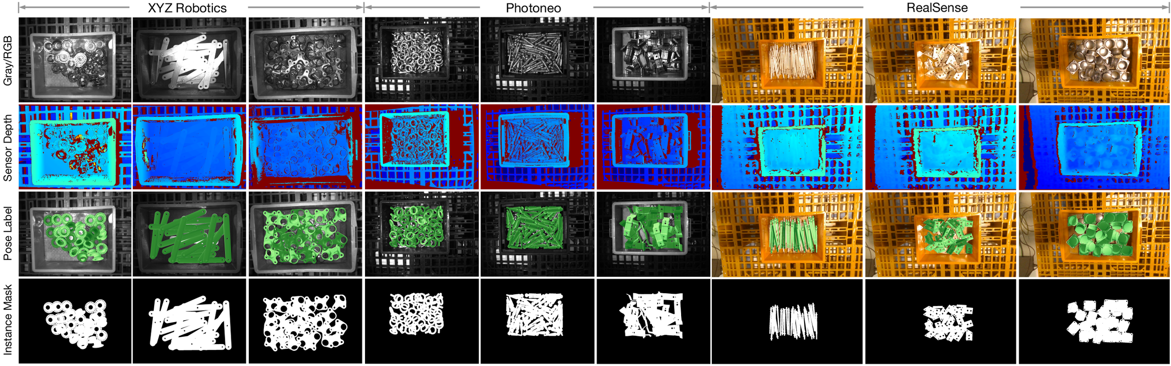
XYZ-IBD mounts RealSense, DLP structured-light, and Photoneo sensors on a FANUC arm to capture 75 dense bin scenes of 15 reflective, textureless, highly symmetric industrial parts. The ECCV-accepted version reports 22.5K frames and around 273K pose instances. Depth captured with antireflection spray, multiview fusion, manual coarse registration, and multiscale ICP establish labels. BOP 6D detection AP is only 0.266 for GDRN, 0.247 for SurfEmb, 0.564 for FoundationPose, and 0.578 for SAM6D, well below BOP-Core 5. Reported 0.999 mm / 0.432° accuracy comes from simulated error quantification reproducing noise and annotation steps. The project page retains an older 91K-annotation count; use v3 / ECCV statistics and identify the version.
RealSense RGB-DXYZ Robotics DLP grayscale and structured-light depthPhotoneo grayscale and laser-triangulation depthaligned raw and anti-reflection capturesCAD models, instance masks and 6D posesBlenderProc synthetic RGB-D training set
Requirements
known industrial object CAD modelscalibrated camera intrinsics and robot-camera extrinsicsBOP-compatible detector or instance masksRGB-D sensing for geometry-aware baselinessymmetry definitions for MSSD / MSPD evaluation
Full paper metadataAuthors, affiliations, research area, datasets, metrics, method tags, and reading statusExpandCollapse
Authors
Junwen Huang, Jiaqi Hu, Peter KT Yu, Slobodan Ilic, Martin Sundermeyer, Benjamin Busam
Affiliations
Technical University of Munich / Munich Center for Machine Learning / XYZ Robotics / ROBOX / Google
known industrial object CAD modelscalibrated camera intrinsics and robot-camera extrinsicsBOP-compatible detector or instance masksRGB-D sensing for geometry-aware baselinessymmetry definitions for MSSD / MSPD evaluation
Reading Notes
Overview / Deep Dive
Available src/paper-notes/xyz-ibd-eccv2026/coarse.md
Paper overview notes
Quickly assess the paper's scope, problem setting, core method, experimental findings, and whether to read it in depth.
XYZ-IBD introduces a benchmark rather than a new pose network, moving 6D pose evaluation from relatively tidy household objects to real industrial bins: 15 reflective, textureless, often symmetric parts recur in 75 densely stacked scenes. The ECCV accepted version reports about 22.5K frames and 273K pose instances. Three sensors, two-pass capture with temporary anti-reflection coating, and multiview CAD registration generate accurate labels; BOP baselines show substantial degradation for both seen and unseen methods.
2.1 Guide to the paper’s figures and tables
Figure / table
What to inspect first
Supported conclusion
Unsupported inference
Figure 2
Grayscale / RGB, raw depth, poses, and masks from XYZ DLP, Photoneo, and RealSense
The data cover multiple sensors, reflections, and dense instances
Multiple sensors in the dataset do not require simultaneous three-camera input at inference
Figure 6
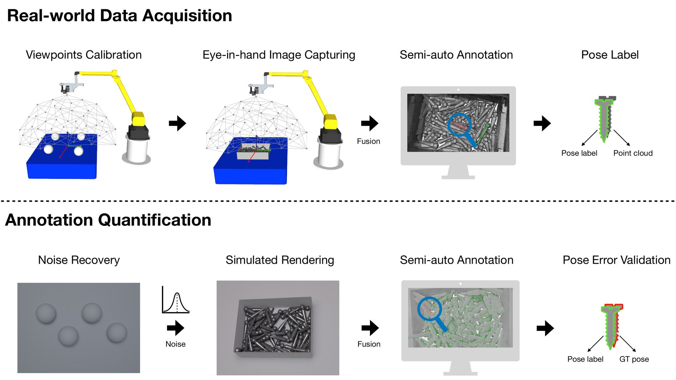
Separate real capture and simulated error-quantification pipelines
Label generation and accuracy validation are separate processes
Small simulated errors do not provide independently measured physical GT for every real scene
Figure 7
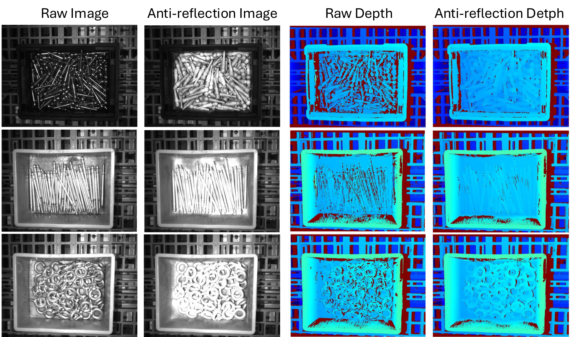
Depth before and after anti-reflection coating
Coating substantially fills depth gaps on metal surfaces
Label-generation observations are not extra test-time inputs
Figure 10
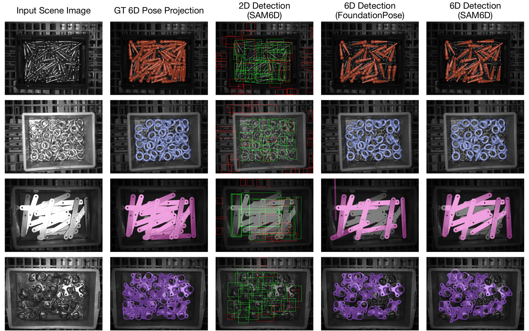
SAM6D and FoundationPose detection / 6D pose visualizations
Repeated instances, occlusion, and reflection damage both detection and pose
Qualitative images cannot replace the tabulated symmetry-aware AP
Original Figure 2: three sensor groups correspond to XYZ Robotics DLP, Photoneo, and RealSense; rows show grayscale / RGB, sensor depth, pose projections, and instance masks. Source: arXiv. Image copyright belongs to the authors and publisher; reproduced here for paper analysis.
Setting: real industrial bin picking; many repeated instances share one CAD model, with random stacking, heavy occlusion, and strong reflections.
Objects: 15 metal industrial parts, approximately 54–300 mm in diameter, mostly textureless and geometrically symmetric.
Real data: 75 scenes, with 5 rearrangements per object; the text reports 11–60 instances per scene, averaging about 22.
Training data: about 45K RGB-D frames generated by physical free-fall simulation in BlenderProc, with masks, depth, and 6D poses.
Outputs: confidence-scored instance masks; or 6D detections comprising object identity, rotation, and translation.
Setup: both seen-object and unseen-object evaluation, within a model-based benchmark with known CAD.
Important boundaries
Unseen object means no object-specific retraining on these 15 instances; CAD / rendered templates remain available at test time. This is not unrestricted open-world pose without references.
Anti-reflection coating is used only to generate high-quality GT depth and pose labels. Public test inputs retain the original reflective appearance; methods cannot use the ideal coated depth at inference.
The main contribution is the benchmark and annotation protocol. The best AP in the table should not be presented as a new SOTA method proposed by the authors.
4. Core motivation
On household datasets such as YCB-V, texture, semantics, and lower instance density allow many methods to approach saturation.
Industrial parts often look nearly identical in color and texture, with many repeated instances. Detectors struggle with instance boundaries, while pose networks lack stable appearance cues.
Specular reflection saturates RGB and causes extensive missing or distorted structured-light and stereo depth.
Symmetry and occlusion create multiple solutions, while bin picking generally tolerates much smaller positional errors than household AR scenarios.
If GT itself is derived from reflection-corrupted depth, the benchmark confounds sensor bias with algorithm error; an independent label-generation path is therefore needed.
5. Dataset construction overview
5.1 Capture hardware
Device
Main outputs
Reported specifications / role
FANUC M10iD/8L
Repeated positioning at 50 viewpoints
±0.06 mm repeatability
Intel RealSense D415
1920×1080 RGB + stereo depth
General RGB-D baseline modality, 30 FPS
XYZ Robotics AL-M DLP
1440×1080 grayscale + structured-light depth
0.08 mm depth resolution; primary annotation camera
Photoneo PhoXi M
Grayscale + laser-triangulation depth
Up to 2064×1544; 0.1 mm voxel precision
All three cameras are rigidly mounted on the robot wrist, at a working distance of about 600–1000 mm.
5.2 Multiview calibration
Place 4 precision spheres on the working plane.
Randomly sample 50 viewpoints on a hemisphere at elevations of 45°–90°.
Perform camera undistortion and hand-eye calibration.
Refine the 6DoF transforms from 49 secondary views to the primary view using ICP on sphere point clouds.
The paper reports mean calibration RMSE of about 0.248 mm.
5.3 Two-pass capture and annotation
First apply temporary Acksys SP-102 coating to suppress metal reflections and obtain more complete depth.
Wait about 15 minutes at 25°C±1°C for the coating to evaporate, then revisit the same viewpoints to capture the original reflective appearance.
Fuse coating-enhanced depth across views into a unified scene cloud.
Annotators roughly align CAD models in a constrained GUI using ±1 mm / ±1° increments, followed by multiscale ICP from downsampled to full resolution.
Propagate primary-camera poses through calibrated extrinsics to all 50 viewpoints and the other two cameras, avoiding manual per-frame alignment.
Original Figure 6: the upper pipeline covers viewpoint calibration, eye-in-hand multiview capture, semiautomatic CAD alignment, and pose propagation. The lower pipeline recovers noise in simulation, repeats annotation, and compares against known GT poses. Source: arXiv. Image copyright belongs to the authors and publisher; reproduced here for paper analysis.Original Figure 7: raw depth on reflective metal contains many holes and discontinuities; temporary anti-reflection coating produces more complete surface depth. Enhanced depth is used only for fusion and labels, without replacing raw test observations. Source: arXiv. Image copyright belongs to the authors and publisher; reproduced here for paper analysis.
5.4 Error quantification
The authors cannot directly obtain more accurate physical GT for every real stacked scene, so they reproduce the full process in simulation:
Add Gaussian noise to depth from 50 calibration views; at σ=0.26 mm, ICP calibration RMSE is 0.248 mm, matching the real system.
Generate randomly stacked scenes in BlenderProc and apply the recovered noise model.
Run the same multiview fusion, manual adjustment, and ICP annotation on simulated scenes.
Match annotated poses to simulated GT by 3D centroid using Hungarian assignment.
Report mean position error of 0.999 mm (standard deviation 0.12 mm) and angular error of 0.432° (standard deviation 0.08°).
This supports approximately 1 mm / 1° accuracy, but it is an error estimate from a simulated reproduction of the process, not direct metrology of every real label. At 0.999 mm, the mean is only just below 1 mm and should not be described as far below a millimeter.
6. Dataset statistics and version conventions
The ECCV accepted v3 / Table 1 reports:
75 real scenes;
22.5K frames;
About 273K annotated instances;
15 objects;
An average of 22 instances per scene-image, up to 60;
45K synthetic training frames.
However, the public project page still lists “22K images, 91K annotations, average 24 instances.” The split section reports 2,250 validation frames + 9,000 test frames. Although 91K × 3 equals 273K, the paper does not fully reconcile camera, two-pass, frame, and annotation counting levels. These notes adopt the latest ECCV / arXiv v3 figure of 273K while retaining the version discrepancy. Specify versions when building tables or inspecting download manifests; do not mix older project-page counts.
7. Experimental overview
7.1 Protocol
2D detection: COCO-style AP averaged over mask IoU 0.50–0.95 in increments of 0.05.
6D detection: BOP 2024–2025 symmetry-aware AP aggregated over MSSD and MSPD correctness thresholds.
Seen methods: train on the XYZ-IBD synthetic split, then evaluate on the real test split.
Unseen methods: use externally pretrained large-scale models directly, without XYZ-IBD fine-tuning.
Unseen pose methods share SAM-6D masks; seen pose methods use YOLOX detections.
7.2 Baseline results
Method
Task
Unseen objects
BOP-Core 5 AP
XYZ-IBD AP
Change
YOLOX
2D detection
No
0.798
0.774
-0.024
CNOS
2D detection
Yes
0.361
0.275
-0.086
SAM-6D detector
2D detection
Yes
0.449
0.296
-0.153
NIDS-Net
2D detection
Yes
0.494
0.258
-0.236
GDRN
6D detection
No
0.827
0.266
-0.561
SurfEmb
6D detection
No
0.758
0.247
-0.511
MatchU
6D detection
Yes
0.705
0.529
-0.176
FoundationPose
6D detection
Yes
0.734
0.564
-0.170
SAM6D
6D detection
Yes
0.704
0.578
-0.126
Original AP values are from Table 4; changes were calculated here relative to BOP-Core 5.
Seen pose methods are especially notable: despite synthetic training on the target CAD, GDRN and SurfEmb drop from 0.827 / 0.758 to 0.266 / 0.247. Unseen RGB-D + CAD registration is stronger, but even the best SAM6D reaches only 0.578, leaving the benchmark unsolved.
Original Figure 10: left to right are input, GT pose projection, SAM6D 2D detection, and FoundationPose / SAM6D 6D detection. Green / red boxes denote correct / incorrect object IDs. Dense repeated instances cause missed detections, identity errors, and incomplete pose outputs. Source: arXiv. Image copyright belongs to the authors and publisher; reproduced here for paper analysis.
8. Strengths and limitations
Strengths
Goes beyond adding images by jointly emphasizing reflections, symmetry, repeated instances, random stacking, and heavy occlusion.
Three sensors and repeatable robot positioning provide a multimodal, reproducible capture foundation.
Coating-enhanced depth produces labels while original reflective observations serve testing, keeping GT generation separate from test conditions.
BOP-compatible seen / unseen 2D and 6D detection protocols connect readily to mainstream methods.
Public synthetic training, validation, test images, CAD, and leaderboard access support practical use.
Limitations / risks
Only 15 objects, with limited coverage of the full industrial material and geometry distribution.
Real-label accuracy is mainly estimated by simulated reproduction, without independent per-instance CMM / tracker validation of real stacked poses.
The “sub-millimeter” mean is 0.999 mm: mathematically valid wording with very little margin.
The public project page, ECCV v3, and split section use incompletely reconciled frame / annotation counts.
Seen and unseen pose methods use different detection / mask priors, so AP gaps cannot be attributed entirely to pose backbones.
Training relies primarily on synthetic-to-real transfer; high YOLOX 2D AP does not establish successful real-domain pose correspondence.
Data use CC BY-NC-SA 4.0; commercial industrial use requires separate license clarification.
9. Research takeaways
Reusable idea: temporary surface treatment for GT generation while retaining original optical conditions for testing can help label transparent / reflective objects.
Suitable baseline? A priority benchmark for industrial bin picking, reflective objects, and dense-instance pose; good YCB-V results alone are insufficient.
Worth deep reading? Yes, especially capture, calibration, annotation error, and BOP evaluation.
Open questions: can multisensor self-supervision replace coating? Can independent CMM validate real-label errors? How can detection, mask, and pose failures be separated?
Available src/paper-notes/xyz-ibd-eccv2026/deep.md
In-depth paper notes
Support reproduction, comparison, related-work writing, and identifying opportunities for further research.
Deep Reading Notes: XYZ-IBD: Benchmarking Robust 6D Object Pose Estimation under Real-World Industrial Complexity
Reading focus: whether industrial difficulty has verifiable causes, how anti-reflection two-pass capture generates labels, what error quantification establishes, and whether baseline degradation arises in detection or pose.
2. Positioning in one sentence
XYZ-IBD benchmarks model-based 2D / 6D object detection for real industrial bin picking: 15 reflective, textureless, often symmetric metal parts are densely and randomly stacked. The ECCV accepted version reports 75 scenes, about 22.5K frames, and 273K pose instances. Labels combine three sensors, repeatable robot viewpoints, temporary anti-reflection coating, coarse CAD alignment, and multiscale ICP. Existing seen and unseen methods both degrade substantially under industrial complexity.
My central assessment
The contribution combines three often separate industrial pose problems in one benchmark: dense repeated instances, reflection-degraded observations, and assembly-level accuracy requirements. Ordinary benchmarks can yield high scores under mild occlusion, distinguishable appearance, or limited label precision. XYZ-IBD asks where each instance is, whether it matches the target CAD, and whether its pose is accurate enough under symmetry equivalence.
An easily overstated claim needs qualification: 0.999 mm / 0.432° are errors against known simulated GT after reproducing sensor noise, calibration, fusion, manual adjustment, and ICP. They support roughly 1 mm / 1° accuracy for the annotation process, rather than independent physical measurement of all 273K real poses. The margin between 0.999 mm and 1 mm is tiny; “far below a millimeter” would overstate it.
2.1 Guide to the paper’s figures and tables
Figure
Content
Evidence provided
Unsupported interpretation
Figure 2
XYZ DLP, Photoneo, and RealSense images, raw depth, poses, and masks
Three-sensor multimodal data with dense instance annotations
Inference requires all three cameras, or multiple sensors inherently guarantee pose accuracy
Figure 6
Real capture and simulated error-quantification pipelines
Separates label generation from error estimation
Simulated validation equals individual metrology of real labels
Figure 7
Raw and coated images / depth
Shows reflective-metal depth gaps and improved fusion after coating
Test methods may use coating-enhanced depth
Figure 10
GT, SAM-6D detection, FoundationPose and SAM6D poses
Illustrates missed instances, wrong IDs, and pose errors
A few qualitative images establish overall method rankings
Original Figure 2: three sensor groups correspond to XYZ Robotics DLP, Photoneo, and RealSense; rows show grayscale / RGB, raw sensor depth, pose projections, and instance masks. Source: arXiv. Image copyright belongs to the authors and publisher; reproduced here for paper analysis.
3. Problem setting and task boundaries
3.1 Four evaluation tasks
Following the BOP 2024–2025 model-based setting, the benchmark has four quadrants:
Task
Object setting
Information available at test time
Representative baselines
2D detection
Seen object
Trained on synthetic data for the 15 target CAD models
YOLOX
2D detection
Unseen object
Target CAD / rendered templates, without XYZ-IBD fine-tuning
CNOS, SAM-6D detector, NIDS-Net
6D detection
Seen object
Target-object synthetic training, with YOLOX frontend
GDRN, SurfEmb
6D detection
Unseen object
General pretrained model + target CAD, with SAM-6D masks
MatchU, FoundationPose, SAM6D
Here, unseen object does not mean open-world pose without CAD. Target 3D models remain known at test time; methods simply are not retrained on XYZ-IBD’s 15 instances. The precise interpretation is model-based pose for unseen instances / novel objects with known CAD.
3.2 6D pose outputs
The target transform for each instance can be written as:
Tco=[Rco0tco1]∈SE(3),
Here Rco and tco transform CAD object-frame points into the camera frame. Full 6D detection also requires object IDs, confidence, and recovery of all visible instances in one image. Unlike single-instance pose with perfect crops or GT masks, missed detections never reach pose solving and directly reduce AP.
3.3 Inputs, outputs, and essential priors
Stage
Inputs
Outputs
Essential priors / dependencies
2D detector
Public test RGB-D (specific methods may use RGB only) + target CAD / templates
Correct CAD scale, frames, and symmetry annotations
3.4 Boundaries of coated data
Temporary anti-reflection coating is label-generation infrastructure: more complete depth enables multiview fusion and CAD alignment. Original reflective observations remain public benchmark inputs. Reading ideal coated depth at test time would leak GT-generation information into inference and prevent fair comparison with the reported baselines.
3.5 Multiple sensors do not imply multisensor inference
The three cameras primarily:
Cover complementary RGB, grayscale, stereo, structured-light, and laser-triangulation observations;
Propagate primary-camera labels to other sensors through rigid mounting and relative extrinsics;
Support research on sensor-domain differences.
They do not require benchmark submissions to fuse all three streams. Inputs must follow the specific task and release protocol; Figure 2 alone does not establish a joint multicamera pose method.
4. Research context
4.1 What household-object benchmarks established
LineMOD, LM-O, YCB-V, HomebrewedDB, and TUD-L established standard model-based pose tasks. HOPE adds robotic manipulation, IC-BIN explores bin picking, and StereoOBJ-1M scales RGB labels using SfM and calibration targets. NOCS and later work such as HouseCat6D expand to category-level pose, new instances, and more complex materials.
These datasets advanced textureless objects, occlusion, symmetry, and synthetic training, but differ in semantics, instance density, and assembly requirements. High household-object scores do not ensure reliable grasp-level pose when many identical metal parts occlude one another and depth is largely missing.
4.2 Gaps in existing industrial data
The paper compares industrial datasets by object count and shape diversity, size, frames, instances, image density, accurate GT depth, occlusion, reflectance, and label error.
T-LESS has 30 textureless, sometimes symmetric industrial objects, but reflective, densely filled random bins are not its main focus.
ITODD includes industrial shapes and challenging lighting, without centering on repeated instances filling bins.
DIMO and ROBI are closer to metal bin picking but have relatively limited object counts or shape coverage.
IPD includes RGB-D, polarization, and industrial parts, with less overall clutter, stacking, and occlusion.
StereOBJ-1M has many images and labels but lacks depth and has limited object diversity.
XYZ-IBD’s added value is the combination of 15 industrial CAD models, an average of 22 and up to 60 instances, strong reflections, three sensors, and an approximately 1 mm annotation process, rather than dominance on one dimension.
4.3 Relationship to BOP
BOP-compatible data and 2D / 6D detection protocols connect XYZ-IBD to template matching, 2D segmentation, RGB correspondence, RGB-D registration, and novel-object pose. It adds an industrial evaluation domain rather than replacing BOP Core datasets.
Table 4’s BOP-Core 5 averages LM-O, T-LESS, YCB-V, IC-BIN, and TUD-L. It covers neither all BOP datasets nor a controlled material comparison. Cross-dataset gaps indicate broad domain difficulty rather than causal effects of an isolated factor.
5.1 Repeated instances defeat the semantic-detection shortcut
Identical parts share category and appearance. Detectors must identify the CAD while separating touching and overlapping instances. A foreground region containing adjacent instances injects structured outliers into later 2D–3D correspondence or cloud registration.
5.2 Reflections corrupt both RGB and depth
Highlights cause saturation and view-dependent appearance changes; stereo or active depth may contain holes, flying points, and biases. This disrupts synthetic-to-real appearance consistency for RGB-only methods and removes geometric alignment evidence for RGB-D registration.
5.3 Symmetry invalidates a unique-orientation assumption
Bolts, pins, covers, and rotational parts may have discrete or continuous symmetry. Direct rotation-matrix comparison can incorrectly reject equivalent geometry. XYZ-IBD uses symmetry-aware MSSD / MSPD, but symmetry handling resolves evaluation ambiguity rather than restoring occluded surfaces or instance boundaries.
5.4 Texture is not the only synthetic-to-real bottleneck
45K synthetic frames vary free fall, materials, and lighting, but cannot easily reproduce real metal BRDFs, active illumination, depth failures, minor wear, and physical contact. Degradation despite target-CAD training shows that knowing geometry does not resolve the observation-domain gap.
5.5 Industrial tolerances amplify label errors
Millimeter-scale GT bias can obscure method differences. Such errors affect contact during assembly, insertion, and grasp approach. Calibration, fusion, and error quantification therefore matter alongside image count.
6. Dataset construction in detail
6.1 Objects and scenes
15 real industrial parts, approximately 54–300 mm in diameter, including sheet-metal parts, bolts, pins, covers, and other machined components.
Industrial partners provide CAD reportedly accurate at micron level. CAD-source accuracy does not establish micron-level accuracy for the entire image-annotation process.
5 real bin rearrangements per object yield 75 scenes.
Each scene has 11–60 heavily overlapping instances, with a reported mean of about 22.
Sensor-to-object distance is about 600–1000 mm, resembling factory layouts.
Table 1 reports 22.5K frames and 273K instances. Mixing cameras, capture passes, or view levels changes the meaning of “per scene” and “per image”; reuse should follow the downloaded manifest’s actual hierarchy.
6.2 Hardware system
Device
Outputs / specifications
Role in the data pipeline
FANUC M10iD/8L
±0.06 mm positioning repeatability
Revisit 50 calibrated viewpoints for coated / raw two-pass capture
Intel RealSense D415
1920×1080 RGB and stereo depth, 30 FPS
Common RGB-D modality representing general-purpose / consumer observations
XYZ Robotics AL-M DLP
1440×1080 grayscale and structured-light depth; reported 0.08 mm depth resolution
Primary annotation camera providing dense coated-surface depth
Photoneo PhoXi M
Grayscale and laser-triangulation depth; up to 2064×1544, 0.1 mm voxel precision
Another industrial 3D sensing domain
All three cameras are rigidly mounted on the robot wrist. Sensor resolution, voxel precision, robot repeatability, and final pose-label accuracy are distinct; neither adding them nor taking their minimum establishes GT accuracy.
6.3 Multiview sampling and calibration
The authors sample 50 viewpoints on a hemisphere centered on the bin, at elevations of 45°–90°, balancing visibility and robot reachability. Calibration proceeds as follows:
Place 4 precision-machined spheres on the working plane;
Undistort cameras and initialize camera poses through hand-eye calibration;
Capture sphere point clouds at each viewpoint;
Refine 6DoF transforms from 49 secondary views to the primary reference using ICP;
Store inter-view transforms for multiview fusion and pose projection.
The text reports mean viewpoint calibration RMSE near 0.248 mm, while Table 2 lists 0.245 mm overall. Both indicate about 0.25 mm; these notes retain the source discrepancy rather than selecting one as definitively more precise.
6.4 Two-pass capture: separating label and test observations
Metal is difficult for active depth. The authors first apply temporary Acksys SP-102 anti-reflection coating and capture high-quality depth. After about 15 minutes at 25°C±1°C for evaporation, the robot revisits the same viewpoints to record original optical appearance.
Ideally the two passes remain spatially aligned within robot repeatability. This offers two advantages:
Labels can rely on complete coated geometry while the benchmark retains real reflective difficulty;
Raw / anti-reflection pairs support depth-restoration and cross-sensor-consistency research.
An implicit assumption is that parts and bins remain entirely static during waiting and revisiting, with no geometry change or displacement from evaporation. Robot ±0.06 mm repeatability constrains camera revisiting, not possible object micromotion between passes.
Original Figure 7: left to right are raw image, anti-reflection image, raw depth, and anti-reflection depth. Coating substantially fills depth gaps on reflective metal; enhanced depth is used only for fusion and labels, without replacing raw test observations. Source: arXiv. Image copyright belongs to the authors and publisher; reproduced here for paper analysis.
6.5 Semiautomatic 6D pose annotation
Labels are not manually dragged into place in every frame. CAD models are aligned once in a unified 3D scene and propagated to all views:
Fuse coating-enhanced multiview depth into one scene cloud;
Adjust CAD in a constrained GUI using ±1 mm translation and ±1° rotation increments;
Run multiscale ICP near the coarse pose, starting with downsampled clouds for larger adjustments and refining at full resolution;
Determine final poses in the XYZ DLP primary camera / reference frame;
Propagate labels to all 50 views using calibrated inter-view transforms;
Project to RealSense and Photoneo using rigid inter-camera extrinsics.
This hierarchy reduces manual work from “each instance × each view × each camera” to once per scene instance. Shared geometric origins improve cross-view consistency, but calibration bias can affect many frames together; more samples do not average away systematic extrinsic errors.
Original Figure 6: the upper pipeline shows 50-view calibration, eye-in-hand capture, multiview fusion, semiautomatic CAD alignment, and label propagation. The lower pipeline recovers noise in simulation, repeats acquisition and annotation, and compares with known GT. Source: arXiv. Image copyright belongs to the authors and publisher; reproduced here for paper analysis.
6.6 Annotation error: what was actually validated
Real scenes lack an obviously more accurate external GT system capable of measuring every occluded part. The authors therefore construct a BlenderProc environment with known truth and estimate accumulated error in three steps.
Step 1: recover equivalent noise
Use the same calibration spheres and camera parameters in simulation, sample 50 viewpoints, and add Gaussian noise of varying standard deviation to rendered depth. Run comparable ICP calibration to relate noise to viewpoint-calibration RMSE:
Gaussian depth noise σ(mm)
calibration RMSE (mm)
0.00
0.199
0.10
0.209
0.20
0.233
0.26
0.248
0.30
0.259
At σ=0.26 mm, RMSE is 0.248 mm, close to real calibration. The authors adopt this as equivalent noise for accumulated sensor, robot, and multiview calibration effects.
Step 2: reproduce scenes and annotation
Drop identical CAD models into a simulated bin, render noisy multiview data, and rerun fusion, manual adjustment, and multiscale ICP. Known simulated poses allow direct comparison between annotation outputs and GT.
Step 3: match instances and measure pose error
Using 3D-centroid distance as cost, Hungarian assignment matches generated labels to GT. Analysis uses up to 60 samples per scene across 3 scenes for each object. Reported errors are:
Mean translation error 0.999 mm, standard deviation 0.12 mm;
Mean rotation error 0.432°, standard deviation 0.08°.
What this validation supports
Under the authors’ equivalent Gaussian noise, simulated geometry, and reproduced annotation conditions, mean process error is near 1 mm / 0.43°. This is more convincing than sensor specifications or ICP residual alone.
It does not directly establish that:
Every real label has error below 1 mm; a below-threshold mean does not bound the tail;
Gaussian noise fully models real reflective-depth holes, flying points, or spatially correlated biases;
CAD tolerances, wear, and micromotion during coating / evaporation have been independently measured;
0.999 mm and 0.432° can be collapsed into a single accuracy score.
Calling 0.999 mm sub-millimeter is numerically valid but leaves almost no margin. A careful conclusion is “mean translation error of approximately 1 mm, estimated through simulated reproduction.”
6.7 Synthetic training set
For each object, 120 free-fall simulations produce 25 rendered frames per scene, with randomized materials, lighting, instance count, and poses. This yields about 3,000 frames per object and about 45K RGB-D samples overall, with instance masks, depth, and 6D poses.
These samples supervise seen-object baselines on target CAD rather than adding real-scene training labels. They expose sim-to-real performance: models have seen target geometry but not identically distributed real training images.
6.8 Real splits, released content, and counting issues
The split section reports:
Validation: 15 scenes, 2,250 frames;
Test: 60 scenes, 9,000 frames;
Synthetic training: about 45K frames;
Sizes of approximately 80 GB synthetic, 8 GB validation, and 3 GB test;
Public test images, GT hosted on an evaluation server, and released training / validation annotations and CAD.
However, Table 1 reports 22.5K real frames, while older project text lists 22K images, 91K annotations, and an average of 24 instances. 2,250 + 9,000 = 11,250 differs from 22.5K by a factor of two; 91K × 3 = 273K also matches the sensor count, without a unified explanation in the text.
These notes use 22.5K / 273K from the latest ECCV / arXiv v3 as the paper’s main figures, while retaining unresolved questions:
Does frame count both raw and anti-reflection passes?
Does annotation count projections across all three sensors?
Is the project page’s 91K from an earlier dataset version?
How are images, scenes, and cameras organized in the actual download manifest?
Before training or publishing statistics, count the downloaded files and record the release version rather than mixing paper and project-page figures.
6.9 License boundaries
The project page specifies CC BY-NC-SA 4.0 and directs commercial users to request a custom license. Academic use still requires attribution and share-alike compliance; an industrial subject does not imply permission for commercial deployment, products, or training combined with internal production data.
7. Evaluation protocol in detail
7.1 2D detection AP
2D tasks output nonoverlapping binary instance masks and confidence. COCO-style AP uses mask IoU thresholds 0.50, 0.55, …, 0.95, aggregating precision over thresholds and objects.
This is stricter than IoU 0.5 alone: dense touching instances may have roughly correct regions yet fail high-IoU thresholds. Mask quality also affects RGB crops, visible point clouds, and correspondences in pose pipelines.
7.2 6D detection AP
The paper uses BOP 2024–2025 symmetry-aware MSSD and MSPD.
For CAD surface points M, equivalent symmetry transforms S, predicted pose P^, and GT pose P, MSSD can be summarized as:
eMSSD=S∈Sminx∈MmaxP^x−PSx2.
It measures worst-case 3D surface-point deviation after symmetry equivalence. MSPD instead projects transformed points into the image:
eMSPD=S∈Sminx∈Mmaxπ(P^x)−π(PSx)2,
Here π denotes camera projection. Final AP aggregates objects, error types, and multiple correctness thresholds.
The metrics complement each other: MSSD emphasizes 3D alignment and physical manipulation, while MSPD emphasizes image projection. Symmetry sets permit only predefined equivalents; incorrect metadata or unmodeled approximate symmetry can still make scores diverge from practical graspability.
7.3 Comparison conditions are not identical
Seen 2D / pose methods train on synthetic target-CAD data;
Unseen methods use externally pretrained large-scale weights without XYZ-IBD fine-tuning;
Seen pose methods use a YOLOX frontend;
Unseen pose methods share SAM-6D masks.
Table 4 therefore compares complete systems under their standard settings, rather than isolating seen / unseen pose backbones. Masks, training scale, RGB / RGB-D modalities, and refinement computation all differ.
8. Results and interpretation
8.1 Complete Table 4
Method
Task
Unseen objects
YCB-V
T-LESS
LM-O
BOP-Core 5
XYZ-IBD
Absolute change
YOLOX
2D detection
No
0.877
0.707
0.894
0.798
0.774
-0.024
CNOS (SAM)
2D detection
Yes
0.490
0.395
0.330
0.361
0.275
-0.086
SAM-6D detector (SAM)
2D detection
Yes
0.518
0.465
0.437
0.449
0.296
-0.153
NIDS-Net
2D detection
Yes
0.650
0.496
0.439
0.494
0.258
-0.236
GDRN
6D detection
No
0.906
0.852
0.775
0.827
0.266
-0.561
SurfEmb
6D detection
No
0.799
0.828
0.760
0.758
0.247
-0.511
MatchU
6D detection
Yes
0.756
0.668
0.680
0.705
0.529
-0.176
FoundationPose
6D detection
Yes
0.889
0.646
0.756
0.734
0.564
-0.170
SAM6D
6D detection
Yes
0.845
0.515
0.699
0.704
0.578
-0.126
Absolute changes are calculated here as XYZ-IBD - BOP-Core 5; original AP comes from Table 4. These are cross-benchmark score differences rather than relative percentage changes.
8.2 2D detection: seen and unseen methods diverge
YOLOX falls from 0.798 to 0.774, just 0.024, showing that synthetic supervision on 15 target objects can preserve strong class / instance detection. Dense-instance detection is not thereby easy:
YOLOX is evaluated on fixed seen objects;
Synthetic training and real testing share CAD models;
Correct 2D masks / detections do not require millimeter-level 3D poses.
All three unseen detectors degrade, with NIDS-Net falling furthest to 0.258. SAM proposals, rendered templates, and visual feature matching encounter repeated appearances, highlights, and occlusion, affecting both candidate regions and CAD-identity ranking.
8.3 Seen 6D pose: target-CAD training remains insufficient
GDRN drops from 0.827 to 0.266, and SurfEmb from 0.758 to 0.247, the largest declines in the table. This strongly supports benchmark difficulty: a detector at 0.774 AP can still feed correspondence / regression stages that fail under reflection, occlusion, and sim-to-real gaps.
GDRN uses dense RGB-RoI 2D–3D correspondences, surface regions, and visible masks with Patch-PnP; SurfEmb learns surface embeddings. Both require stable links between observed appearance and synthetic supervision. View-dependent metal highlights, mutual occlusion, and small visible surfaces break those links.
8.4 Unseen RGB-D registration is relatively more robust
MatchU, FoundationPose, and SAM6D reach 0.529, 0.564, and 0.578 respectively, clearly above the two seen pose baselines. They center on CAD, RGB-D, and general features / registration, relying less on target-specific RGB pose regression.
This single table does not show that unseen methods always outperform seen methods:
The three unseen methods share SAM-6D masks, unlike the seen frontend;
They typically use heavier rendering, matching, coarse-to-fine, or refinement procedures;
No controlled experiment standardizes masks, runtime, and compute;
Even the best 0.578 remains far from reliable industrial operation.
8.5 What qualitative results reveal about failures
Original Figure 10: left to right are input, GT pose projection, SAM-6D 2D detection, and FoundationPose / SAM6D 6D detection; green / red boxes indicate correct / incorrect object IDs. Source: arXiv. Image copyright belongs to the authors and publisher; reproduced here for paper analysis.
Figure 10 helps build a failure taxonomy rather than replace quantitative tables:
Missed detections: severely occluded instances lack masks and never reach pose estimation;
Wrong IDs: similar metal parts or partial contours match incorrect CAD models;
Mixed masks: one region covers adjacent instances, creating structured registration outliers;
Rotation ambiguity: symmetric or near-symmetric parts yield plausible poses outside GT equivalence;
Translation drift: depth holes and occlusion displace CAD along surface normals or axes;
Local success with poor overall recall: a few good overlays cannot compensate for many omitted instances; AP penalizes both precision and recall.
8.6 Claims versus evidence
Author claim
Direct evidence
My assessment
Real industrial complexity
Industrial robot / sensors, 15 metal parts, 75 real rearrangements, average 22 / maximum 60 instances
Well supported, but 15 objects cannot cover all industrial materials and processes
Sub-mm / sub-degree labels
Simulated process mean 0.999 mm / 0.432°
Supports approximately 1 mm / 1° process-level mean estimates, not strict per-real-instance bounds
Harder than existing benchmarks
AP comparison for 9 baselines on BOP-Core 5 and XYZ-IBD
Supports increased overall difficulty, without factorwise causal ablations of material, occlusion, or density
Holds for these complete systems; different masks, training, and compute preclude a single-architecture explanation
Suitable open benchmark
BOP-compatible tasks and data / CAD / leaderboard plans
Sensible engineering direction; reproduction still requires release manifests, count versions, and server-status checks
9. Critical assessment
9.1 Main strengths
Combined difficulty factors
Many datasets emphasize one factor such as transparency, reflection, occlusion, or scale. XYZ-IBD combines difficult factors in bins of repeated instances, preventing detectors and pose estimators from relying on background, semantic category, or a single complete outline.
Clear separation of annotation and test conditions
Coating-enhanced depth generates GT; raw reflective images define the benchmark. This is more credible than ICP labels from reflection-corrupted depth and closer to deployment than providing specially treated surfaces at test time.
Process-level validation of accuracy claims
The authors reproduce calibration, fusion, manual adjustment, and ICP before comparison with known simulated GT, rather than equating sensor resolution with label accuracy. Despite limited extrapolation, this is stronger than inferring good GT from small ICP residuals.
Shared BOP seen / unseen protocols
Joint reporting of 2D and 6D detection helps locate frontend and backend bottlenecks. Novel-object methods with known CAD can enter evaluation without retraining on 15 objects.
9.2 Main limitations
No independent physical metrology of real labels
A single Gaussian standard deviation fitted to calibration RMSE may miss spatial correlations, material-dependent holes, thermal drift, and multipath effects. Industrial sub-mm metrology would benefit from independent checks on sampled visible instances using CMM, optical trackers, or fixtures with known poses, reporting median, 95th percentile, and maximum errors.
Limited object and material coverage
15 objects support dense instances but cannot represent transparent plastics, dark absorbing parts, flexible objects, cables, mixed materials, scratches, and manufacturing tolerances. The paper’s object diversity +++ is a qualitative author rating, not a standardized statistic.
Scenes appear dominated by repeated copies of one CAD
Five rearrangements per object aid same-object bin-picking research, but mixed-SKU similarity, incorrect CAD retrieval, and long-tail inventory need separate evaluation. Similar-size parts with matching local geometry would couple object identity more strongly to pose.
Different frontends and compute across seen / unseen systems
YOLOX and SAM-6D provide different masks; RGB regression and RGB-D registration also consume different inputs. Without GT-mask upper bounds, standardized proposals, or runtime / memory tables, detection, pose, and depth-corruption contributions cannot be precisely separated.
Version inconsistencies in dataset counts
22.5K, 11.25K, 273K, 91K, and averages of 22 / 24 instances coexist. Camera, pass, and version counting may explain this without erroneous data, but a benchmark paper should explicitly decompose dimensions such as scene × arrangement × viewpoint × sensor × pass × modality.
No controlled difficulty bins
Table 4 establishes overall difficulty but lacks AP curves by visibility, instance density, symmetry, reflectance, sensor, depth completeness, or size. Such breakdowns would help prioritize masks, features, geometric registration, or uncertainty calibration.
9.3 Potential hidden biases
Although 50 robot views are sampled on a hemisphere, the manifest is needed to assess strongly correlated viewpoints or shared backgrounds across train / validation / test.
Poses propagate to many views, but only 75 independent physical configurations underlie the large frame count; image count is not effective sample size.
Synthetic and real data share exact CAD, testing model-based generalization within a closed geometry set rather than missing CAD, scanning errors, or manufacturing differences.
In centroid-based Hungarian label-error matching, close same-object centers may affect assignment stability; matching-threshold sensitivity is not reported.
10. Reproduction and usage checklist
10.1 Minimum inputs
Official release’s 15 CAD models, scales, and object frames;
Per-sensor intrinsics, distortion parameters, and inter-camera extrinsics;
Synthetic training, real validation, and test-image manifests;
Official BOP 2024–2025 2D / 6D detection evaluator;
Table 4 baseline weights, template-rendering parameters, and score thresholds.
10.2 Initial data-integrity checks
Count files by scene, view, camera, pass, and modality to reconcile 22.5K and 11.25K;
Count pose instances by object, camera, and split to reconcile 273K and 91K;
Randomly project CAD into RGB / depth to verify intrinsics, extrinsics, and millimeter units;
Check pixel / 3D alignment between raw and anti-reflection captures;
Verify symmetry transforms against canonical CAD frames;
Ensure local training and tuning never access test GT;
Record download date, release tag, and license text.
10.3 Fair baseline comparisons
Report at least three result levels:
GT masks + pose backend, estimating the pose-stage upper bound;
One detector / mask source + different backends, isolating backend capability;
Official complete pipelines, measuring practical usability.
Include per-image latency, GPU memory, template preprocessing costs, and refinement iterations. Industrial bin picking needs throughput; AP alone cannot establish deployability.
10.4 Recommended diagnostic bins
Variable
Why it matters
Recommended visualization
Visible surface ratio
Directly quantifies occlusion
AP–visibility curve
Instances per image
Separates ordinary clutter from dense stacks
AP–density curve
Raw-depth valid ratio
Isolates reflection effects on registration
AP–depth completeness curve
Symmetry type
Separates continuous, discrete, and asymmetric objects
Grouped MSSD / MSPD AP
Sensor
Compares consumer and industrial depth domains
Three-sensor table
Object diameter / visible pixels
Identifies small-object and distance issues
Scale-binned AP
GT versus predicted masks
Separates detection from pose
Oracle-mask gap
11. Further research directions
11.1 Multisensor consistency to reduce coating dependence
Depth sensors fail differently across materials. Cross-sensor consistency, known robot motion, and CAD renders could supervise depth / normal recovery on raw reflective surfaces, reducing surface-treatment costs during labeling.
11.2 Explicit depth invalidity and uncertainty
Rather than filling missing depth indiscriminately, predict per-pixel validity and anisotropic noise, propagating uncertainty into correspondence weighting, PnP / registration, and pose covariance. Robots can then choose to grasp, change viewpoint, or abstain.
11.3 Joint instance-segmentation and pose association
A segment-then-pose cascade can lock in a wrong mask among dense identical instances. Multiple joint segmentation–pose hypotheses could use CAD-render consistency, visible surfaces, and nonpenetration to revise instance boundaries.
11.4 Physical bin constraints
Parts must remain inside the bin, avoid substantial interpenetration, and satisfy gravitational stability. Multi-instance pose optimization can incorporate these constraints when single-view evidence is ambiguous, especially for rotational symmetry or heavy occlusion.
11.5 Active viewpoint planning
XYZ-IBD’s 50 viewpoints suit next-best-view research. Pose hypotheses, symmetry ambiguity, and missing depth could guide the next camera position rather than forcing acceptance of a difficult view.
11.6 Propagating real-label uncertainty
Benchmarks need not provide only one GT pose. Calibration covariance, ICP Hessians, visible surfaces, and symmetry could estimate per-label SE(3) uncertainty, avoiding overconfident point labels for inherently ambiguous scenes.
11.7 From single SKU to mixed SKU and CAD retrieval
Warehouses often mix similar parts. Joint evaluation of CAD-library retrieval, unknown rejection, and pose would expose object-ID errors otherwise hidden by predefined candidate sets.
12. Practical research implications
For synthetic-to-real research
Randomize more than texture and light: simulate active-depth holes, flying points, view-dependent highlights, and sensor types, then calibrate noise against real raw / anti-reflection pairs.
For novel-object pose research
XYZ-IBD provides a more discriminative stress test than household data. Report known CAD, depth usage, mask source, refinement iterations, and template counts instead of grouping different compute budgets under one zero-shot label.
For detection or segmentation research
An average of 22 and maximum of 60 same-object instances supports proposal-recall, boundary, and object-ID calibration studies. Besides AP, report GT / predicted counts per image, crowded-region recall, and ID-confusion matrices.
For robotic grasping research
BOP AP is necessary but insufficient as a proxy. Feed poses to a grasp planner and report collision rate, grasp success, placement error, and decision latency. Grasp equivalence for symmetric objects may differ from visual symmetry sets.
For building a dataset
The key reusable design separates four roles: high-quality annotation observations, realistic test observations, shared robot poses, and independent error reproduction. Strengthen it with limited external real-label metrology and transparent dimension-wise counts.
13. Overall assessment
Contribution strength
XYZ-IBD offers an industrial-domain stress test and annotation engineering solution. Fifteen objects provide limited category coverage, but 75 real rearrangements, dense repeated instances, raw reflections, three sensors, and BOP-compatible seen / unseen evaluation expose systematic failures that household benchmarks may conceal.
Evidence credibility
Difficulty: strong. Hardware, scenes, Figures 2 / 7, and cross-benchmark AP degradation support one another.
Annotation pipeline: strong. Calibration, coating, fusion, manual adjustment, and ICP are clearly described.
Real-label sub-mm claim: moderate. Simulated validation exceeds specification-based inference but lacks direct physical-GT sampling; 0.999 mm leaves little margin.
Method comparison: moderately strong. Table 4 covers representative seen / unseen systems without fully standardized frontends and computation.
Reproducibility: depends on completeness of releases, evaluation server, version manifests, and baseline configurations.
Recommended use
Make XYZ-IBD a priority benchmark for industrial bin picking, reflective / textureless parts, dense multi-instance pose, novel-object RGB-D registration, or pose uncertainty. Beyond overall AP, informative experiments include oracle masks, standardized frontends, visibility / depth-validity bins, and real-robot success.
Brief conclusion
Even with known CAD, target-object synthetic training, and powerful general pretrained models, real reflective metal bins substantially reduce 6D detection AP. XYZ-IBD provides a convincing annotation engineering approach, but approximately 1 mm denotes a simulated process-level mean estimate, not physical certification of every real label.